Code
source("R/flower_glyphs.R")
plants <- load_plants()TidyTuesday 2026-02-03 · The Edible Plant Database (GROW Observatory)
The Edible Plant Database describes 146 food crops by their growing requirements — sunlight, water, feeding, soil pH, time to harvest. That’s k-dimensional data crying out for a multivariate display.
The classic answer is a Chernoff face: map each variable to a facial feature and let human face-perception do the pattern-matching. Faces are powerful but faintly absurd for vegetables. So this page borrows Chernoff’s idea and the shape of Fisher’s iris measurements (petal length, petal width, counts) but grows flower glyphs instead — each crop rendered as the bloom its growing conditions imply.
source("R/flower_glyphs.R")
plants <- load_plants()Every glyph is a faithful encoding of five growing variables. Nothing is decorative:
| Flower feature | Variable | Meaning |
|---|---|---|
| Number of petals | Sunlight | 5 = shade-tolerant · 6 = sun/part-shade · 8 = full sun |
| Petal length | Days to harvest | longer petals = slower crop |
| Petal width | Water need | fatter petals = thirstier |
| Centre size | Feeding (nutrients) | bigger golden disc = hungry feeder |
| Petal colour | Soil pH | acid-blue → neutral-violet → alkaline-pink (a hydrangea’s logic) |
decoder <- tibble(
  common_name = c("Quick · sun · thirsty · hungry",
                  "Slow · sun · dry · lean",
                  "Shade · medium · acid soil",
                  "Slow · part-shade · alkaline"),
  sun_lvl = c("Full sun", "Full sun", "Shade-tolerant", "Sun or part shade"),
  harvest_days = c(30, 160, 90, 150),
  water_lvl = c(5, 1, 3, 2),
  nutrient_lvl = c(3, 1, 2, 2),
  ph_mid = c(6.4, 6.4, 5.3, 7.6)
)

draw_garden(build_garden(decoder, ncol = 4), label_size = 3) +
  labs(title = "Four reference blooms",
       subtitle = "Read every real flower below against these")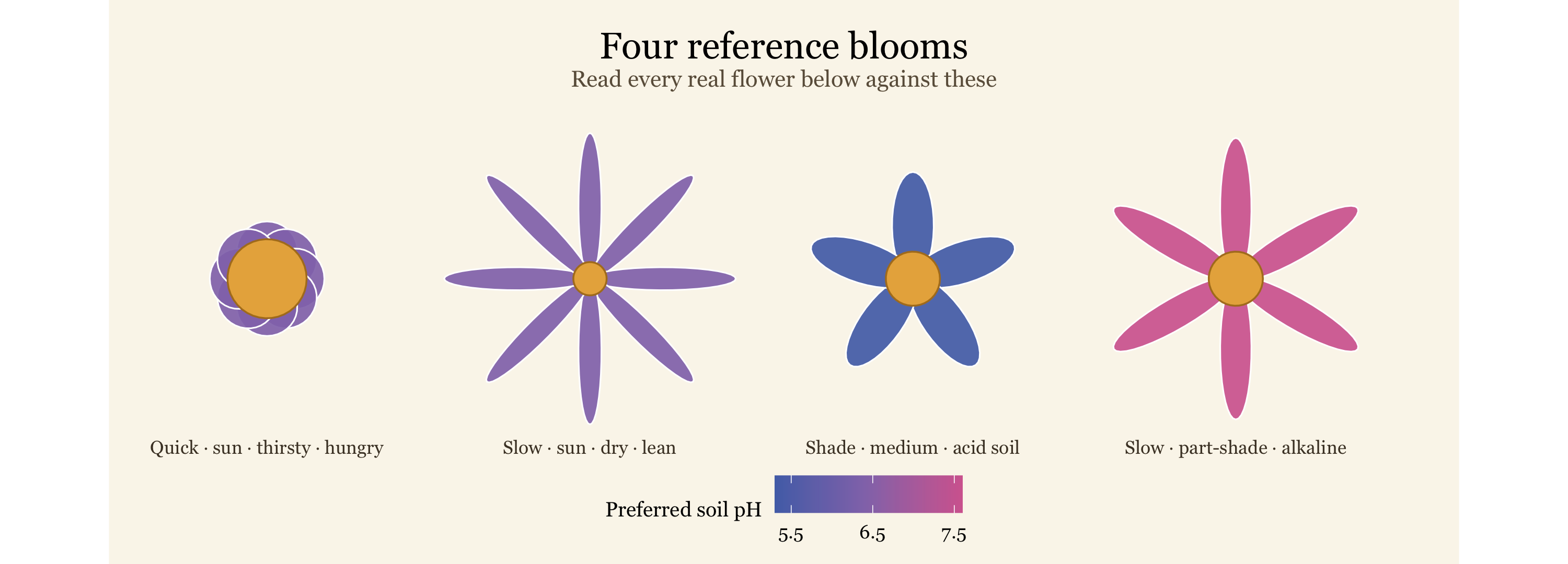
A selection of common kitchen-garden crops, sorted left-to-right, top-to-bottom by time to harvest — so the bloom-size visibly swells as you read down the plot, from the radish that’s ready in three weeks to the cucumber and leek that make you wait.
wanted <- c("Radish", "Spinach", "Lettuce (Headed)", "Rocket", "Beetroot",
  "Pea", "Mangetout", "Carrot", "Kale", "Broccoli", "Cauliflower",
  "Bell Pepper", "Chilli Pepper", "Tomato (Cherry)", "Garlic", "Fennel",
  "Sweetcorn", "Celery", "Beans (Runner)", "Pumpkin", "Onion", "Parsnip",
  "Cucumber", "Leek")

garden <- plants |>
  filter(common_name %in% wanted,
         !is.na(harvest_days), !is.na(ph_mid),
         !is.na(water_lvl), !is.na(nutrient_lvl)) |>
  arrange(harvest_days)

draw_garden(build_garden(garden, ncol = 6)) +
  labs(
    title = "A kitchen garden, encoded",
    subtitle = "Petals = sunlight · length = days to harvest · width = water · centre = feeding · colour = pH"
  )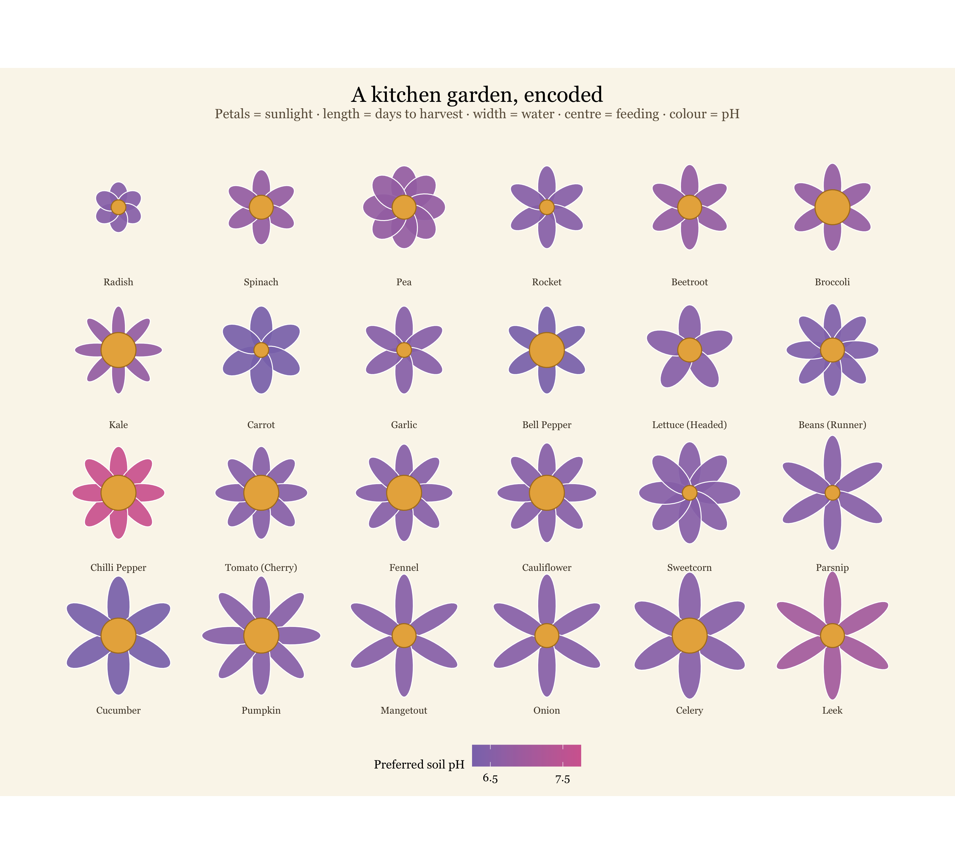
The flower form does what Chernoff intended — it turns rows of numbers into gestalts you can sort by eye:
plants |>
  filter(!is.na(water_lvl), !is.na(nutrient_lvl)) |>
  count(water_lvl, nutrient_lvl) |>
  ggplot(aes(water_lvl, nutrient_lvl, size = n)) +
  geom_point(colour = "#7a9a4e", alpha = 0.8) +
  scale_size_area(max_size = 16, name = "species") +
  scale_x_continuous(breaks = 1:5,
    labels = c("very low", "low", "medium", "high", "very high")) +
  scale_y_continuous(breaks = 1:3, labels = c("low", "medium", "high")) +
  labs(
    title = "Thirsty crops do tend to be hungry crops",
    subtitle = "The glyphs' coupling of petal width and centre size reflects a genuine association",
    x = "Water requirement", y = "Nutrient requirement"
  ) +
  theme_minimal(base_size = 12)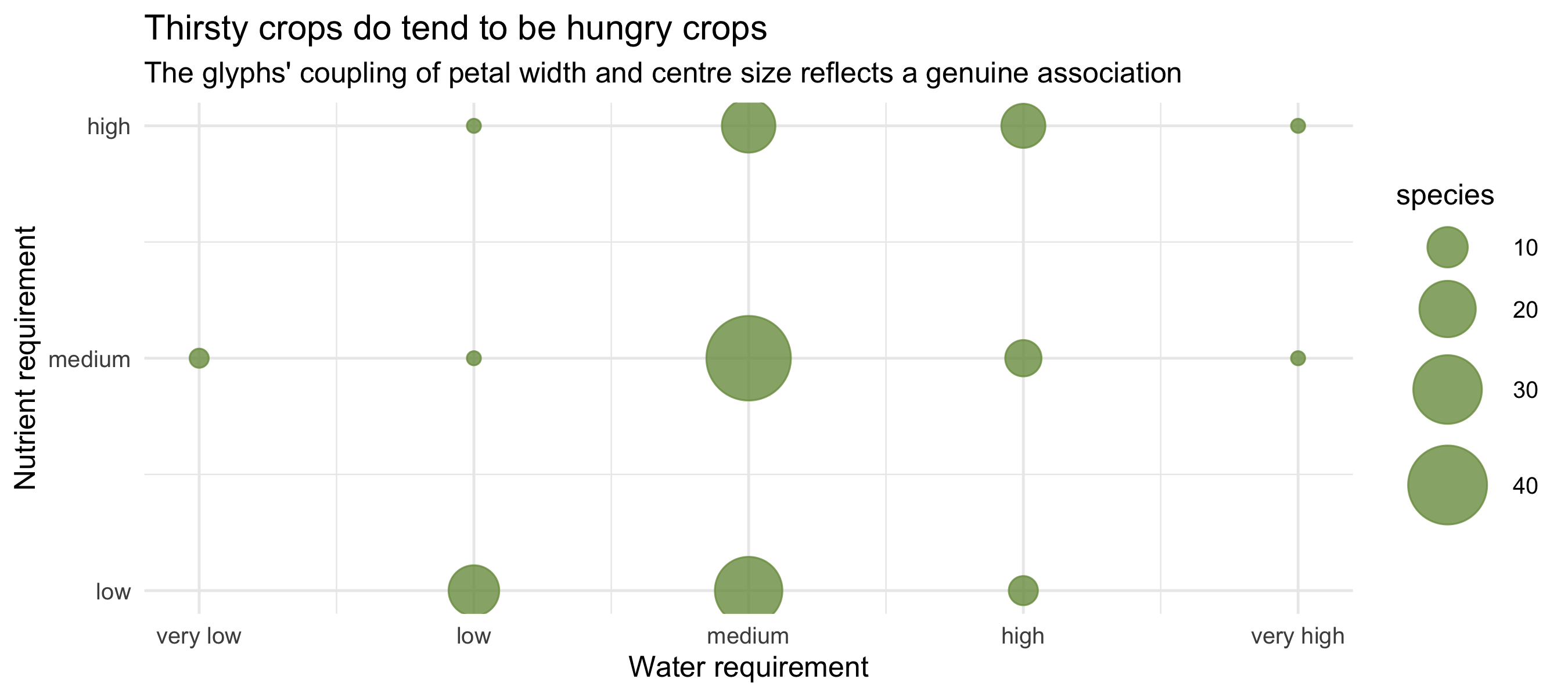
The glyph display isn’t just decoration: the eye’s impression that fat-petalled flowers have big centres turns out to be a real positive association between water and nutrient demand. That is exactly the Chernoff bet — that a well-chosen visual mapping lets pattern-recognition find structure faster than a correlation table would.
Glyph displays trade precision for gestalt. Petal count is the strongest visual signal but encodes only a 3-level variable (sunlight), while the subtle pH colour does heavy lifting that’s easy to miss. As with Chernoff faces, which feature carries which variable changes what pops — assign the loudest channel to the variable you most want compared.