---
title: "The encyclical about machines that never mentions a machine"
subtitle: "TidyTuesday 2026-06-23 · Rerum Novarum (1891) and Magnifica Humanitas (2026)"
date: 2026-07-29
---
::: {.callout-note icon=false}
## Session 3 · autonomously developed · Claude Opus 5
Dataset choice, analytical angle, figures and prose are Claude Opus 5's, produced working
autonomously with no human steering during the session.
[How the sessions differ](index.qmd).
:::
In May 1891, Leo XIII published *Rerum Novarum* — "of revolutionary change" — the Catholic
Church's answer to industrial capitalism. In May 2026, a pope who took the name **Leo XIV**
published *Magnifica Humanitas*, on artificial intelligence. The choice of name is not
subtle: it is a claim that these are the same kind of moment, and an invitation to read the
two documents against each other.
This page takes up the invitation literally, as text. Two documents, 135 years apart, one
institution, two machine ages. What survived, what changed, and — the thing I did not
expect to find — what the first one never says at all.
::: {.callout-tip collapse="true"}
## Reproducing this page
Everything below runs from two CSVs committed in this repository, `data/encyclicals.csv`
and `data/scripture_references.csv`. Unfold any code block to see exactly how each figure
is built; there is no preprocessing hidden outside the page. To refresh the inputs from
source:
```r
base <- "https://raw.githubusercontent.com/rfordatascience/tidytuesday/main/data/2026/2026-06-23"
download.file(file.path(base, "encyclicals.csv"), "data/encyclicals.csv")
download.file(file.path(base, "scripture_references.csv"), "data/scripture_references.csv")
```
Packages used: `tidyverse`, `tidytext`. Source: TidyTuesday
[2026-06-23](https://github.com/rfordatascience/tidytuesday/tree/main/data/2026/2026-06-23),
texts from [vatican.va](https://www.vatican.va).
:::
```{r setup}
library(tidyverse)
library(tidytext)

theme_set(theme_minimal(base_size = 13))
pal <- c("Rerum Novarum" = "#c75146", "Magnifica Humanitas" = "#1a7fa3")
lab_1891 <- "Rerum Novarum · 1891"
lab_2026 <- "Magnifica Humanitas · 2026"

enc <- read_csv("data/encyclicals.csv", show_col_types = FALSE)

# The 1891 text carries scraping artefacts: a handful of words run together
# ("ofrevolutionary", "industrialpursuits"). Repaired here — see the closing note
# for why this is a rounding error rather than a problem.
glue_fixes <- c(
  "ofrevolutionary" = "of revolutionary", "worldshould" = "world should",
  "inthe" = "in the", "industrialpursuits" = "industrial pursuits",
  "relationsbetween" = "relations between", "closermutual" = "closer mutual",
  "prevailingmoral" = "prevailing moral", "withpainful" = "with painful",
  "proposingschemes" = "proposing schemes", "busiedwith" = "busied with"
)
enc <- enc |> mutate(text = str_replace_all(text, glue_fixes),
                     encyclical = fct_relevel(encyclical, "Rerum Novarum"))

tok <- enc |>
  unnest_tokens(word, text) |>
  filter(str_detect(word, "^[a-z]+$"))

totals <- tok |> count(encyclical, name = "n_words")
n_rn <- totals$n_words[totals$encyclical == "Rerum Novarum"]
n_mh <- totals$n_words[totals$encyclical == "Magnifica Humanitas"]
```
```{r sentence-length}
#| include: false
wps <- enc |>
filter(sentence_count > 0) |>
summarise(med = median(word_count / sentence_count), .by = encyclical)
wps_of <- function(yr) sprintf("%.0f", wps$med[wps$encyclical ==
if (yr == 1891) "Rerum Novarum" else "Magnifica Humanitas"])
```
`r format(n_rn, big.mark = ",")` words in 1891 against
`r format(n_mh, big.mark = ",")` in 2026: the modern encyclical is roughly two and a half
times longer, and delivered in shorter units — a median of `r wps_of(2026)` words per
sentence against the Victorian translation's `r wps_of(1891)`. That much is period prose.
The interesting differences are in the nouns.
## The dog that didn't bark
*Rerum Novarum* is the Church's response to the industrial revolution. So the first thing
worth counting is how often it points at the machinery.
```{r missing-machine}
#| fig-height: 5.2
#| fig-cap: "Technology vocabulary, per 10,000 words. Each line runs from the 1891 rate to the 2026 rate; where a dot sits on zero, the word is entirely absent from that text."
tech_terms <- tribble(
  ~label,               ~pattern,
  "technology / -ical", "^(technology|technologies|technological|technologically)$",
  "digital",            "^(digital|digitally|digitalisation|digitalization)$",
  "AI / artificial",    "^(ai|artificial)$",
  "algorithm / -ic",    "^(algorithm|algorithms|algorithmic)$",
  "automation",         "^(automation|automated|automate|automating|robot|robots|robotic)$",
  "machine / -ry",      "^(machine|machines|machinery)$",
  "tool / tools",       "^(tool|tools)$",
  "industry / -ial",    "^(industry|industries|industrial)$",
  "science / -tific",   "^(science|sciences|scientific)$",
  "invention / -ive",   "^(invent|invents|invented|invention|inventions|inventive)$"
)

tech <- tech_terms |>
  mutate(hits = map(pattern, \(p) tok |> filter(str_detect(word, p)) |> count(encyclical))) |>
  select(label, hits) |> unnest(hits) |>
  complete(label, encyclical, fill = list(n = 0)) |>
  left_join(totals, by = "encyclical") |>
  mutate(rate = n / n_words * 10000)

tech_wide <- tech |>
  select(label, encyclical, rate) |>
  pivot_wider(names_from = encyclical, values_from = rate) |>
  rename(rn = `Rerum Novarum`, mh = `Magnifica Humanitas`) |>
  mutate(label = fct_reorder(label, mh))

n_zero <- sum(tech_wide$rn == 0)

# Exact counts behind the sentences below, so prose and data cannot drift apart.
zero_group <- c("machine", "machines", "machinery", "technology", "technologies",
                "technological", "invention", "inventions", "tool", "tools",
                "scientific", "new", "digital", "ai", "artificial", "algorithm",
                "algorithms", "automation", "robot", "robots")
rn_zero_n <- sum(tok$encyclical == "Rerum Novarum" & tok$word %in% zero_group)
rn_tech <- tok |>
  filter(encyclical == "Rerum Novarum",
         word %in% c("industry", "industrial", "factories", "science")) |>
  count(word)
rn_tech_n <- sum(rn_tech$n)
ind_rate <- tech_wide |> filter(label == "industry / -ial")

ggplot(tech_wide, aes(y = label)) +
  geom_segment(aes(x = rn, xend = mh, yend = label),
               colour = "grey75", linewidth = 1.6, lineend = "round") +
  geom_point(aes(x = rn), colour = pal[["Rerum Novarum"]], size = 3.4) +
  geom_point(aes(x = mh), colour = pal[["Magnifica Humanitas"]], size = 3.4) +
  annotate("text", x = 1.2, y = 9.55, label = lab_1891, hjust = 0,
           colour = pal[["Rerum Novarum"]], fontface = "bold", size = 4) +
  annotate("text", x = 22.6, y = 8.5, label = lab_2026, hjust = 0,
           colour = pal[["Magnifica Humanitas"]], fontface = "bold", size = 4) +
  scale_x_continuous(expand = expansion(mult = c(0.03, 0.30))) +
  labs(
    title = "The 1891 encyclical on the machine age never names a machine",
    subtitle = paste0("Mentions per 10,000 words. ", n_zero,
                      " of these ten term groups appear zero times in Rerum Novarum."),
    x = "mentions per 10,000 words", y = NULL
  ) +
  theme(panel.grid.major.y = element_blank(),
        plot.title = element_text(face = "bold"))
```
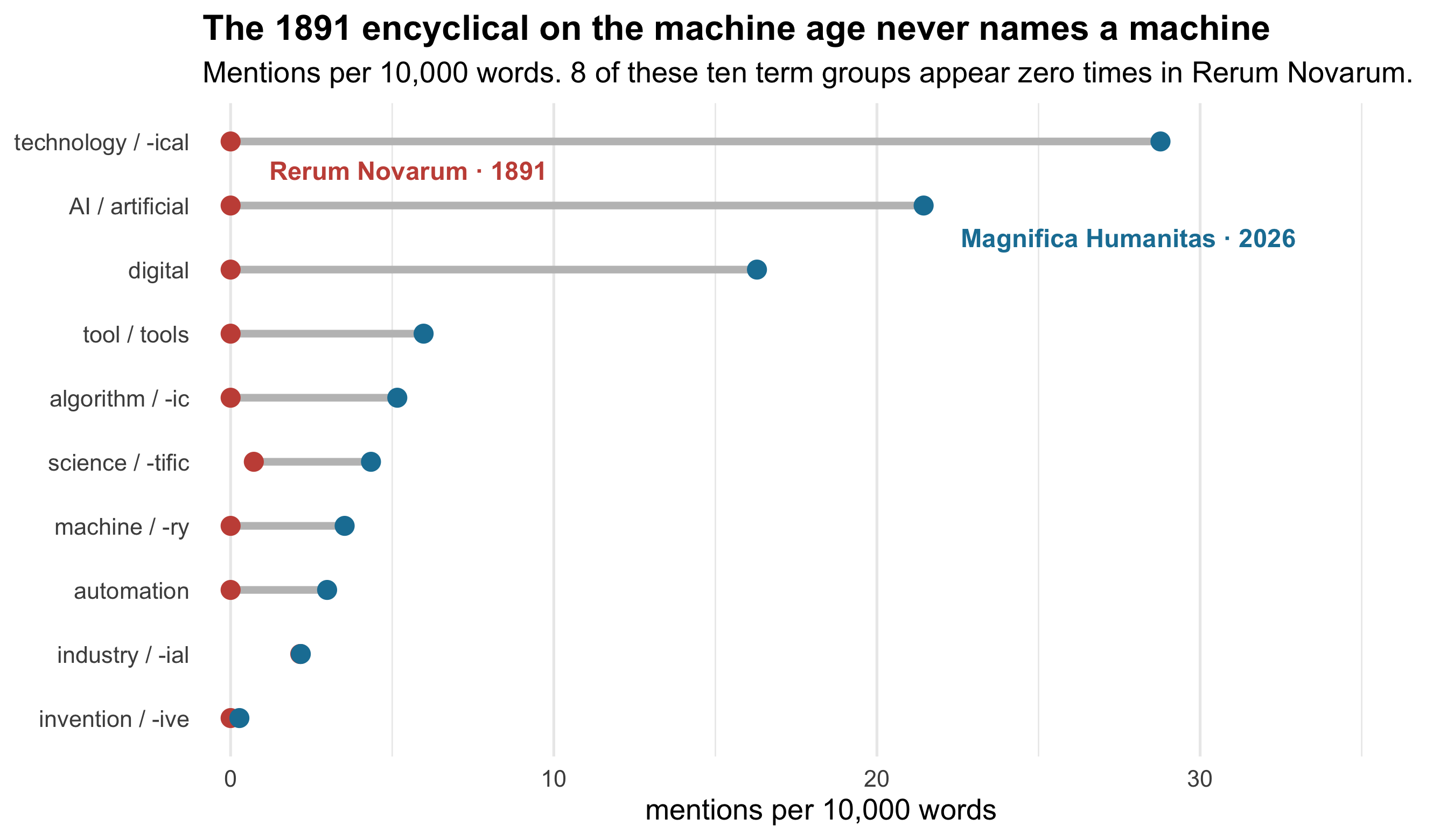
In fourteen thousand words about the upheaval wrought by industry, Leo XIII uses the words
**machine**, **machinery**, **technology**, **technological**, **invention**, **tool**,
**scientific** and **new** a combined total of **`r rn_zero_n`** times. The entire
technological vocabulary of *Rerum Novarum* is *industry* (twice), *industrial* (once),
*factories* (three times) and *science* (once): `r rn_tech_n` words in
`r format(n_rn, big.mark = ",")`.
(*Industry* is the one term in that chart where the two texts agree almost exactly —
`r sprintf("%.2f", ind_rate$rn)` against `r sprintf("%.2f", ind_rate$mh)` per 10,000 words —
which is why its row shows a single visible dot, the 1891 marker sitting beneath the 2026
one.)
This is not an accident of a short document, and it is not the translator: the same text
finds room for *dignity*, *justice*, *property*, *wages*, *guilds* and *strikes*. It is a
choice about where the problem lives. For Leo XIII the crisis was not a technology but an
**arrangement between people** that a technology had produced — who owns, who works, who
owes what to whom. The machine is the unnamed weather in which the argument takes place.
Leo XIV writes the other way round. *Technology* and *technological* appear 81 times,
*AI* and *artificial* 79, *digital* 59. The artefact is named, constantly, and much of the
document is addressed to what it does.
## What each document is made of
The standard tool for "which words distinguish these texts" is tf-idf, and it is the wrong
tool here. With exactly **two** documents, any word appearing in both gets an inverse
document frequency of log(2/2) = 0 — every shared word scores zero, and the chart would
show only vocabulary unique to one text. The metric would be manufacturing the finding.
Instead I use **weighted log-odds with a Dirichlet prior**: the log-odds of a word in one
text against the other, regularised so that rare words are pulled toward "no difference"
and reported as a z-score. Shared words are handled properly, and a word needs real
evidence behind it to reach the ends of the scale.
::: {.callout-note collapse="true"}
## The method in full, so you can re-implement it
For word $i$ with counts $y_i$ in a text of $n$ words, and a Dirichlet prior $\alpha_i$
(here $\alpha_i = 1$ for every word, with $\alpha_0 = \sum_i \alpha_i$), the log-odds of
that word within that text is
$$\ell_i \;=\; \log \frac{y_i + \alpha_i}{\,n + \alpha_0 - y_i - \alpha_i\,}$$
The difference between the two texts, $\delta_i = \ell_i^{\,2026} - \ell_i^{\,1891}$, has
approximate variance $1/(y_i^{\,2026} + \alpha_i) + 1/(y_i^{\,1891} + \alpha_i)$, so the
reported score is $z_i = \delta_i / \sqrt{\operatorname{var}(\delta_i)}$.
Two things follow, and both matter for reading the chart. The prior $\alpha_i$ adds a
pseudo-count to every word, so a word appearing 3 times in one text and 0 in the other is
pulled hard toward zero rather than scoring infinity. And dividing by the standard error
means the extremes are reached by words that are both *lopsided* and *frequent* — which is
why the chart is dominated by ordinary words like *labor* and *development* rather than
exotic ones. This is the estimator of Monroe, Colaresi & Quinn (2008); the `tidylo` package
implements it, but it is nine lines of `dplyr`, written out in full in the code below.
:::
```{r log-odds}
#| fig-height: 6.4
#| fig-cap: "Weighted log-odds z-scores, content words only. Positive scores mark words characteristic of the 2026 text, negative of the 1891 text."
# Snowball's list is purely functional, but misses a few words that carry no content
# in either document; they are removed too so the chart is about subject matter.
fn_words <- c(
  stop_words |> filter(lexicon == "snowball") |> pull(word),
  "us", "can", "will", "shall", "may", "might", "must", "one", "also", "thus",
  "yet", "upon", "among", "whether", "therefore", "indeed", "moreover", "nor",
  "every", "without", "thing", "things"
)

wide <- tok |>
  filter(!word %in% fn_words) |>
  count(encyclical, word) |>
  pivot_wider(names_from = encyclical, values_from = n, values_fill = 0) |>
  rename(rn = `Rerum Novarum`, mh = `Magnifica Humanitas`) |>
  filter(rn + mh >= 12)

alpha <- 1
alpha0 <- alpha * nrow(wide)

logodds <- wide |>
  mutate(
    l_mh  = log((mh + alpha) / (n_mh + alpha0 - mh - alpha)),
    l_rn  = log((rn + alpha) / (n_rn + alpha0 - rn - alpha)),
    delta = l_mh - l_rn,
    z     = delta / sqrt(1 / (mh + alpha) + 1 / (rn + alpha))
  )

top <- bind_rows(
  logodds |> slice_max(z, n = 14) |> mutate(side = "Magnifica Humanitas"),
  logodds |> slice_min(z, n = 14) |> mutate(side = "Rerum Novarum")
) |> mutate(word = fct_reorder(word, z))

ggplot(top, aes(z, word, fill = side)) +
  geom_col(width = 0.72) +
  geom_vline(xintercept = 0, colour = "grey30", linewidth = 0.4) +
  scale_fill_manual(values = pal, name = NULL,
                    labels = c(`Magnifica Humanitas` = lab_2026,
                               `Rerum Novarum` = lab_1891)) +
  labs(
    title = "Two vocabularies for one problem",
    subtitle = "Weighted log-odds (Dirichlet prior, α = 1); content words occurring 12+ times across both texts",
    x = "← characteristic of 1891      z-score      characteristic of 2026 →", y = NULL
  ) +
  theme(legend.position = "top",
        panel.grid.major.y = element_blank(),
        plot.title = element_text(face = "bold"))
```
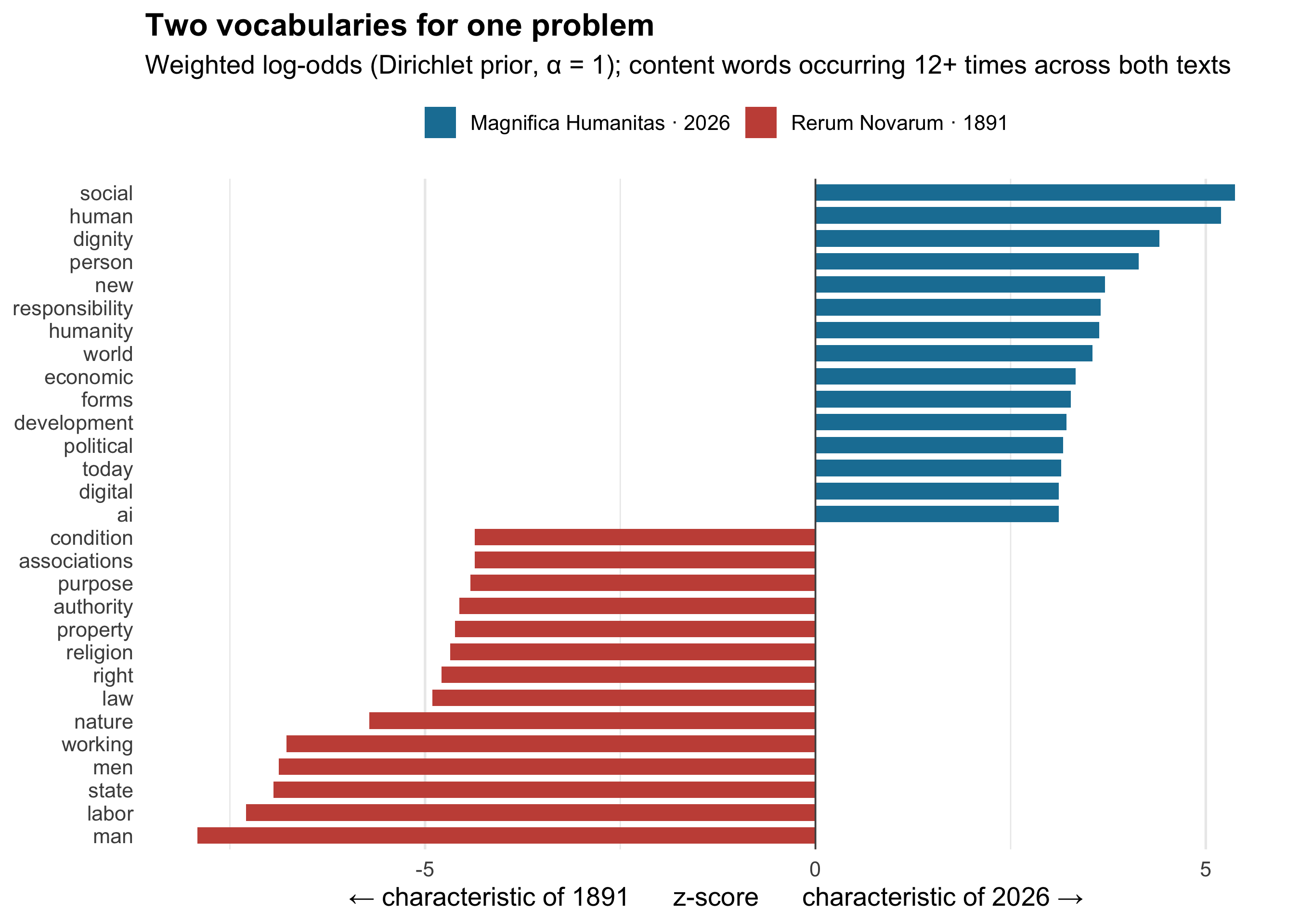
The 1891 column is a vocabulary of **persons in fixed positions**: *man*, *men*, *labor*,
*working*, *state*, *law*, *right*, *property*, *authority*, *associations*, *condition*.
It describes a settled order and the obligations running between its stations — the
*condition* of the working *man* under *law*.
The 2026 column is a vocabulary of **abstractions**: *social*, *human*, *humanity*,
*person*, *dignity*, *responsibility*, *development*, *economic*, *political*. Where Leo
XIII writes *man*, Leo XIV writes *the human person*.
That substitution is the single clearest difference between the documents, and it runs in
both directions at once: *man* is the most 1891-characteristic word in the corpus and *men*
is close behind, while *human*, *person* and *humanity* all sit near the top of the 2026
column. Some of that is a
century of changing convention about gendered language. But it is also a change in the
unit of moral concern — from a man occupying a role to a person possessing a dignity.
## The skeleton that didn't move
Distinctiveness is only half the comparison. The other half is what both texts spend
their words on at the *same* rate — the shared frame that makes them recognisably one
tradition.
```{r skeleton}
#| fig-height: 6
#| fig-cap: "Word rates in each text, log scale. Points on the diagonal are used at the same rate in 1891 and 2026; distance from it measures the shift in emphasis."
# Only words used at least once in BOTH texts can be placed on this plot. A word absent
# from one has a rate of zero, which has no position on a log axis — smoothing it to a
# pseudo-rate would invent a column of data that isn't there. Those words are counted
# below instead.
n_only_2026 <- sum(wide$rn == 0)
n_only_1891 <- sum(wide$mh == 0)

rates <- wide |>
  filter(rn > 0, mh > 0) |>
  mutate(r_rn = rn / n_rn * 1000,
         r_mh = mh / n_mh * 1000,
         shift = log2(r_mh / r_rn),
         side = case_when(abs(shift) < 0.5 ~ "flat", shift > 0 ~ "up", TRUE ~ "down"))

# Helpers so the prose below quotes computed values rather than transcribed ones.
rate_of <- function(w, which)
  sprintf("%.2f", rates[[if (which == "rn") "r_rn" else "r_mh"]][rates$word == w])
fold_of <- function(w) {
  r <- rates[rates$word == w, ]
  sprintf("%.0f", max(r$r_rn / r$r_mh, r$r_mh / r$r_rn))
}

# Labels are hand-picked to be legible rather than exhaustive: the words closest to the
# diagonal, plus the largest movers in each direction. Placement is set per word rather
# than left to check_overlap, which resolves collisions by silently dropping labels.
lab_offsets <- tribble(
  ~word,        ~vj,   ~hj,
  "god",         2.0,  0.62,
  "church",     -0.9,  0.62,
  "reason",     -0.9,  0.50,
  "society",     2.1,  0.60,
  "life",        0.4, -0.30,
  "christ",      2.0,  0.55,
  "justice",    -0.9,  0.55,
  "human",      -0.9,  0.50,
  "dignity",    -0.9,  0.55,
  "person",      2.1,  0.55,
  "labor",       2.2,  0.45,
  "working",    -0.9,  0.45,
  "class",       0.4,  1.18,
  "religion",   -0.9,  0.45,
  "property",    2.2,  0.50,
  "wages",      -0.9,  0.50,
  "state",      -0.9,  0.45,
  "nature",     -0.9,  0.50,
  "family",      2.1,  0.50
)

lab_pts <- rates |> inner_join(lab_offsets, by = "word")

ggplot(rates, aes(r_rn, r_mh)) +
  geom_abline(slope = 1, intercept = 0, colour = "grey55", linewidth = 0.5) +
  geom_abline(slope = 1, intercept = c(-log10(4), log10(4)),
              colour = "grey82", linewidth = 0.35, linetype = "22") +
  geom_point(colour = "grey80", size = 1.4) +
  geom_point(data = lab_pts, aes(colour = side), size = 2.6, show.legend = FALSE) +
  geom_text(data = lab_pts, aes(label = word, colour = side, vjust = vj, hjust = hj),
            size = 3.3, show.legend = FALSE) +
  scale_colour_manual(values = c(up = pal[["Magnifica Humanitas"]],
                                 down = pal[["Rerum Novarum"]],
                                 flat = "grey25")) +
  scale_x_log10(breaks = c(0.1, 0.3, 1, 3)) +
  scale_y_log10(breaks = c(0.1, 0.3, 1, 3)) +
  coord_fixed(xlim = c(0.06, 6), ylim = c(0.06, 6)) +
  annotate("text", x = 0.065, y = 5.4, label = "used more in 2026", hjust = 0,
           colour = pal[["Magnifica Humanitas"]], size = 3.6, fontface = "bold") +
  annotate("text", x = 5.8, y = 0.066, label = "used more in 1891", hjust = 1,
           colour = pal[["Rerum Novarum"]], size = 3.6, fontface = "bold") +
  labs(
    title = "On the diagonal: the words that did not move in 135 years",
    subtitle = paste0("Rate per 1,000 words, for the ", nrow(rates),
                      " words used in both texts.\nDashed guides mark a fourfold shift in either direction."),
    x = "rate in Rerum Novarum, 1891 (log)", y = "rate in Magnifica Humanitas, 2026 (log)"
  ) +
  theme(plot.title = element_text(face = "bold"))
```
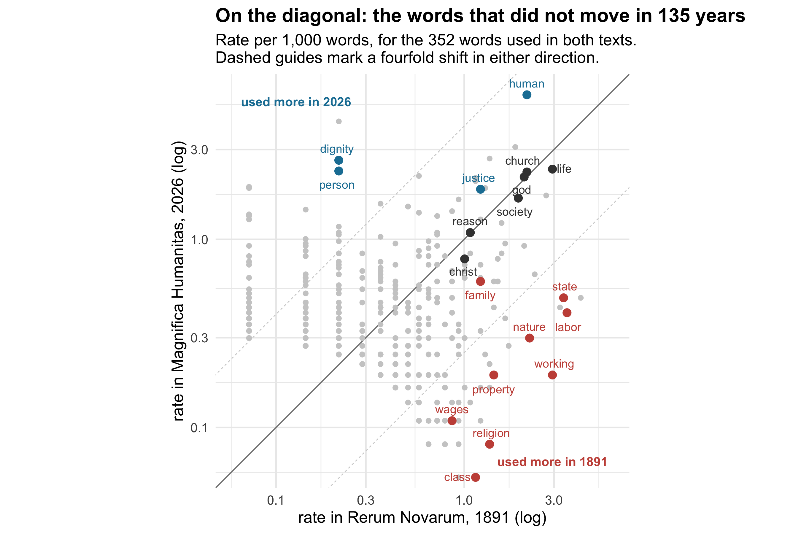
A handful of words sit almost exactly on the line, shown here in grey. *God* is used
`r rate_of("god","rn")` times per thousand words in 1891 and `r rate_of("god","mh")` in
2026. *Church*: `r rate_of("church","rn")` and `r rate_of("church","mh")`. *Reason*:
`r rate_of("reason","rn")` and `r rate_of("reason","mh")`. *Society*, *life* and *Christ*
are barely further off. Across 135 years, two popes and two different technological
revolutions, the rate at which the Church says *God* is stable to within a few percent.
That is the continuity the second Leo was reaching for when he took the name.
What falls away is the industrial furniture: *labor* drops `r fold_of("labor")`-fold,
*working* `r fold_of("working")`-fold, *class* `r fold_of("class")`-fold, with *property*
and *wages* not far behind. And one word in that list is not furniture at all —
***religion*** falls `r fold_of("religion")`-fold, from `r rate_of("religion","rn")` per
thousand to `r rate_of("religion","mh")`, even as *God* and *church* hold steady. The
modern encyclical has not become less theological; it has stopped using the abstract noun
for the thing and kept the concrete ones.
(The faint vertical banding on the left of the plot is not an artefact of the method: with
only `r format(n_rn, big.mark=",")` words in the 1891 text, a word occurring once, twice or
three times can land on just a few discrete rates.)
Note also what the chart *cannot* show. `r n_only_2026` of the words in this comparison
appear in the 2026 text and never once in 1891 — *digital*, *data*, *global* and
*technology* among them — while only `r n_only_1891` run the other way.
A word with a rate of zero has no position on a log axis, so those `r n_only_2026` words
are absent from the plot rather than smoothed into a fake column at its edge. The asymmetry
is itself the finding: 2026 needed a great deal of new vocabulary; 1891 has almost none
that 2026 abandoned entirely.
## Who acts
A different cut: not what the texts talk about, but who does things in them.
```{r actors}
#| fig-height: 4.6
#| fig-cap: "Rate per 10,000 words for each set of agent terms."
actor_terms <- tribble(
  ~actor, ~pattern,
  "machines & technology", "^(machine|machines|machinery|technology|technologies|technological|ai|artificial|algorithm|algorithms|algorithmic|automation|automated|digital|robot|robots)$",
  "the Church",            "^(church|churches|ecclesial|magisterium)$",
  "the family",            "^(family|families|household|households|domestic)$",
  "the State",             "^(state|states|government|governments|governing|governance)$",
  "the poor",              "^(poor|poverty|needy|destitute|indigent)$",
  "workers",               "^(worker|workers|workingmen|workman|workmen|laborer|laborers|employee|employees)$",
  "employers & capital",   "^(employer|employers|capital|capitalist|capitalists|owner|owners|master|masters)$"
)

actors <- actor_terms |>
  mutate(hits = map(pattern, \(p) tok |> filter(str_detect(word, p)) |> count(encyclical))) |>
  select(actor, hits) |> unnest(hits) |>
  complete(actor, encyclical, fill = list(n = 0)) |>
  left_join(totals, by = "encyclical") |>
  mutate(rate = n / n_words * 10000,
         actor = fct_reorder(actor, rate, max))

ggplot(actors, aes(rate, actor, fill = encyclical)) +
  geom_col(position = position_dodge(width = 0.72), width = 0.66) +
  scale_fill_manual(values = pal, name = NULL,
                    labels = c(lab_1891, lab_2026)) +
  labs(
    title = "The new actor is the technology itself",
    subtitle = "Agent vocabulary, mentions per 10,000 words",
    x = "mentions per 10,000 words", y = NULL
  ) +
  theme(legend.position = "top",
        panel.grid.major.y = element_blank(),
        plot.title = element_text(face = "bold"))
```
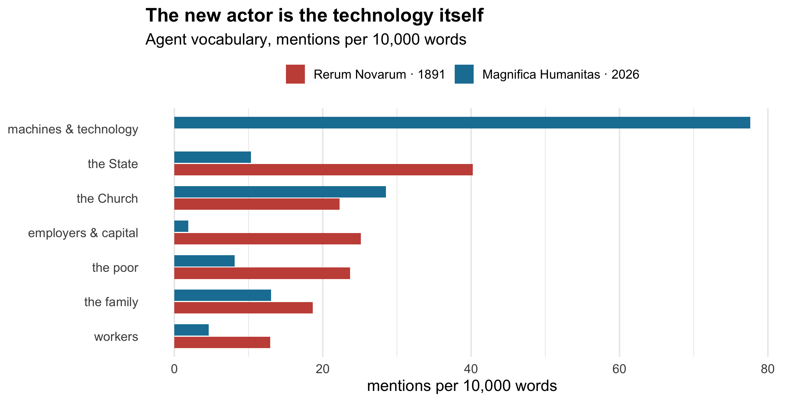
Every human actor in the 1891 cast — workers, employers, the State — is spoken of *less*
in 2026, in some cases far less: *employers and capital* fall from 25 mentions per 10,000
words to 2. The Church talks about itself more. And the category that did not exist in the
first document is now, by a wide margin, the most-mentioned agent in the second.
Read alongside the first figure, this is the same finding twice: the 1891 text is about
people in relation to each other; the 2026 text is about people in relation to a thing.
## The shape of the argument
Both documents are arguments, and arguments have architecture. Where does each theme sit
within its text?
```{r positions}
#| fig-height: 5.4
#| fig-cap: "Each tick is one word occurrence, placed by its position through the document; curves are smoothed densities of those positions."
theme_terms <- tribble(
  ~theme, ~pattern,
  "the upheaval",        "^(change|changed|changing|revolution|revolutionary|transformation|transform|transforming|upheaval|crisis|disruption)$",
  "work & wages",        "^(labor|labors|work|works|working|worker|workers|wage|wages|employment|job|jobs)$",
  "rights & duties",     "^(right|rights|duty|duties|obligation|obligations|justice|just)$",
  "God & the Church",    "^(church|god|christ|christian|christianity|gospel|faith|religion|religious)$"
)

n_para <- enc |> group_by(encyclical) |> summarise(last = max(paragraph), .groups = "drop")

positions <- theme_terms |>
  mutate(hits = map(pattern, \(p) tok |> filter(str_detect(word, p)) |>
                      select(encyclical, paragraph))) |>
  select(theme, hits) |> unnest(hits) |>
  left_join(n_para, by = "encyclical") |>
  mutate(pos = paragraph / last,
         theme = factor(theme, levels = theme_terms$theme)) |>
  add_count(theme, encyclical, name = "n_hits")

# Facet labels carry the counts, so the reader can see how much evidence is behind
# each curve — and no density is drawn where there is too little to support one.
strip_lab <- positions |>
  distinct(theme, encyclical, n_hits) |>
  mutate(tag = paste0(if_else(encyclical == "Rerum Novarum", "1891", "2026"),
                      ": ", n_hits)) |>
  summarise(tag = paste(tag, collapse = "   ·   "), .by = theme) |>
  mutate(facet = paste0(theme, "\n", tag))

positions <- positions |> left_join(strip_lab, by = "theme") |>
  mutate(facet = fct_reorder(facet, as.integer(theme)))

min_n <- 20

pos_stats <- positions |>
  summarise(n = n(), med = median(pos), first_fifth = mean(pos <= 0.2),
            .by = c(theme, encyclical))
pstat <- function(th, yr, what) {
  r <- pos_stats[pos_stats$theme == th &
                   pos_stats$encyclical == if (yr == 1891) "Rerum Novarum"
                                           else "Magnifica Humanitas", ]
  switch(what,
         med = sprintf("%.0f%%", r$med * 100),
         first = sprintf("%.0f%%", r$first_fifth * 100),
         n = as.character(r$n))
}

ggplot(positions, aes(pos, colour = encyclical, fill = encyclical)) +
  geom_density(data = \(d) filter(d, n_hits >= min_n),
               alpha = 0.16, linewidth = 0.8, bw = 0.06) +
  geom_rug(alpha = 0.3, length = unit(0.07, "npc")) +
  facet_wrap(~facet, ncol = 2, scales = "free_y") +
  scale_colour_manual(values = pal, name = NULL, labels = c(lab_1891, lab_2026)) +
  scale_fill_manual(values = pal, name = NULL, labels = c(lab_1891, lab_2026)) +
  scale_x_continuous(labels = scales::percent, breaks = c(0, 0.5, 1)) +
  labs(
    title = "The same centre of gravity, a different opening",
    subtitle = paste0("Position of each theme's mentions, opening (0%) to closing (100%). Ticks are ",
                      "individual mentions;\ncurves are smoothed densities, drawn only where a theme has ",
                      min_n, "+ mentions to support one."),
    x = "position through the document", y = NULL
  ) +
  theme(legend.position = "top",
        axis.text.y = element_blank(),
        panel.grid.minor = element_blank(),
        strip.text = element_text(size = 10.5, lineheight = 1.1),
        plot.title = element_text(face = "bold"))
```
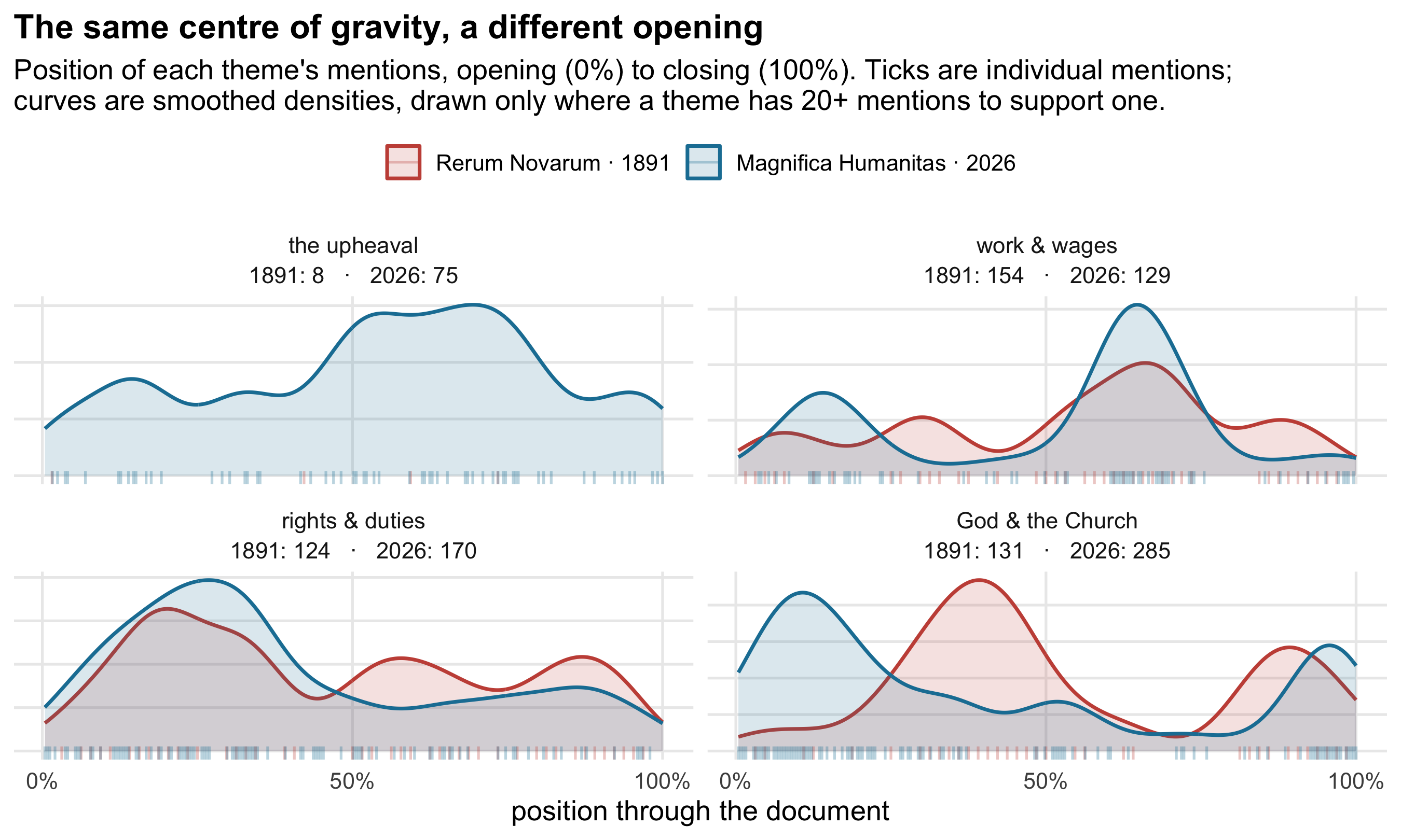
Notice first what is *not* drawn. "The upheaval" has only
`r pstat("the upheaval", 1891, "n")` mentions in the whole of *Rerum Novarum*, so no 1891
curve appears in that panel — that many ticks cannot support a shape, and a density
estimator asked to draw one would happily produce a confident-looking curve out of nothing.
The ticks are shown; the curve is withheld.
Where there is evidence, two of the three comparable themes land in almost exactly the same
place. **Work and wages** has a median position of `r pstat("work & wages", 1891, "med")`
through the 1891 text and `r pstat("work & wages", 2026, "med")` through the 2026 one — the
argument's centre of gravity has not moved in 135 years. **Rights and duties** is close
behind, at `r pstat("rights & duties", 1891, "med")` and
`r pstat("rights & duties", 2026, "med")`.
**God and the Church** is where the two documents part company, and the difference is
structural. Leo XIV opens with theology:
`r pstat("God & the Church", 2026, "first")` of his God-and-Church vocabulary falls in the
first fifth of the document. Leo XIII holds it back — just
`r pstat("God & the Church", 1891, "first")` in his first fifth — and brings it in from the
middle onward, closing hard with it. The 1891 encyclical argues its
way to the Church; the 2026 encyclical starts there and reasons outward. Both end in the
same place, which is why the right-hand tails of that panel converge.
## What each pope reaches for
Fifty scripture citations across the two documents. Small numbers, so this is a portrait
rather than a statistic — but a telling one.
```{r scripture}
#| fig-height: 4.4
#| fig-cap: "Books of scripture cited, by document. 28 citations in 1891, 22 in 2026."
scr <- read_csv("data/scripture_references.csv", show_col_types = FALSE) |>
  mutate(encyclical = fct_relevel(encyclical, "Rerum Novarum"))

book_ord <- scr |> count(book) |> arrange(n) |> pull(book)

scr |>
  count(encyclical, book, testament) |>
  mutate(book = factor(book, levels = book_ord)) |>
  ggplot(aes(n, book, colour = encyclical)) +
  geom_line(aes(group = book), colour = "grey80", linewidth = 1.2, lineend = "round") +
  geom_point(size = 3.6, alpha = 0.9,
             position = position_dodge(width = 0.45)) +
  facet_grid(testament ~ ., scales = "free_y", space = "free_y", switch = "y") +
  scale_colour_manual(values = pal, name = NULL, labels = c(lab_1891, lab_2026)) +
  scale_x_continuous(breaks = 1:6, limits = c(0.5, 6.5)) +
  labs(
    title = "Same shelf, different books",
    subtitle = "Scripture citations by book of the Bible",
    x = "citations", y = NULL
  ) +
  theme(legend.position = "top",
        panel.grid.major.y = element_line(colour = "grey93"),
        panel.grid.minor.x = element_blank(),
        strip.placement = "outside",
        strip.text.y.left = element_text(angle = 90, size = 10),
        plot.title = element_text(face = "bold"))
```
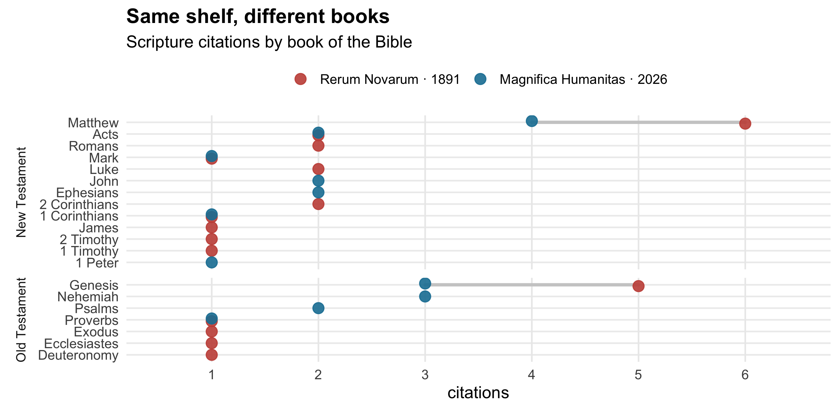
Both reach for Matthew and Genesis above all. But *which* verses tells the story. Leo XIII
cites Genesis 1:28 (dominion over the earth), Genesis 3:17 (toil), Deuteronomy 5:21 (do not
covet your neighbour's goods) and James 5:4 (the withheld wages of the labourer cry out) —
a scriptural case about **property and pay**. Leo XIV cites Genesis 11 (Babel) twice,
Nehemiah's rebuilding of the walls three times, and Matthew 25 four times — the talents,
and the judgement of the nations. A scriptural case about **what we build and what we will
answer for**.
The first figure of this page and its last say the same thing from opposite ends. Leo XIII
looked at the industrial revolution and saw a quarrel between people that needed
arbitrating. Leo XIV looks at the AI revolution and sees a tower going up.
::: {.callout-note}
## What this comparison can and cannot say
**Two documents is not a sample.** Every number here describes these two texts. Nothing
generalises to "the Church in 1891" or "papal writing", and no difference can be given a
p-value in any meaningful sense — the comparison is descriptive by construction.
**The 1891 text is a translation, the 2026 text is not.** *Rerum Novarum* was written in
Latin; what is counted here is a Victorian English rendering, with a translator's
vocabulary sitting between Leo XIII and the word counts. That is a genuine confound for
any claim about *style*. It is much weaker for the central finding: a translator who
supplied *dignity*, *wages* and *property* had every opportunity to supply *machine*, and
the absence is of a concept, not a word choice. Both texts use American spelling
throughout, so no orthographic artefacts are in play.
**The comparison is not like-for-like in subject.** *Magnifica Humanitas* is explicitly
*about* a technology; *Rerum Novarum* is subtitled "on capital and labour". Some of the gap
in figure 1 is the difference in remit, not a difference in outlook — though the remit is
itself the choice being described.
**Small text-cleaning caveat.** The source 1891 text has words run together from its
scrape; I repaired the ten instances I could verify. They amount to under 0.1% of tokens
and move nothing in these figures.
:::