---
title: "Who gets to stay home? European parenting leave, 1970–2024"
subtitle: "TidyTuesday 2026-06-02 · The European Parenting Leave Policies (EPLP) dataset"
date: 2026-06-09
---
::: {.callout-tip icon=false}
## Session 1 · co-developed
This page came out of a live, turn-by-turn conversation between Jon Minton and Claude
(Fable 5) — questions, plots and interpretation built together in real time. The
[Session 2 pages](index.qmd) were instead produced by Claude working autonomously.
:::
A live exploratory session on the [EPLP dataset](https://doi.org/10.5281/zenodo.17648712)
(Spitzer et al. 2025): harmonised parenting-leave regulations for 21 European countries
across 55 years. Durations are in **weeks**; `-98` encodes "not applicable", which we
treat carefully below — for a flat-rate scheme, a missing replacement *rate* is not a
zero, it's a different kind of policy.
```{r setup}
library(tidyverse)

country_names <- c(
  AT = "Austria", BE = "Belgium", CZ = "Czechia", DE = "Germany",
  DK = "Denmark", EE = "Estonia", ES = "Spain", FI = "Finland",
  FR = "France", GR = "Greece", HU = "Hungary", IE = "Ireland",
  IT = "Italy", LT = "Lithuania", NL = "Netherlands", NO = "Norway",
  PL = "Poland", SE = "Sweden", SI = "Slovenia", SK = "Slovakia",
  UK = "United Kingdom"
)

eplp <- read_csv("data/eplp.csv", show_col_types = FALSE) |>
  mutate(
    across(where(is.numeric), \(x) if_else(x == -98, NA_real_, x)),
    across(where(is.character), \(x) na_if(x, "Not applicable")),
    country_name = country_names[country]
  )

theme_set(theme_minimal(base_size = 13))
```
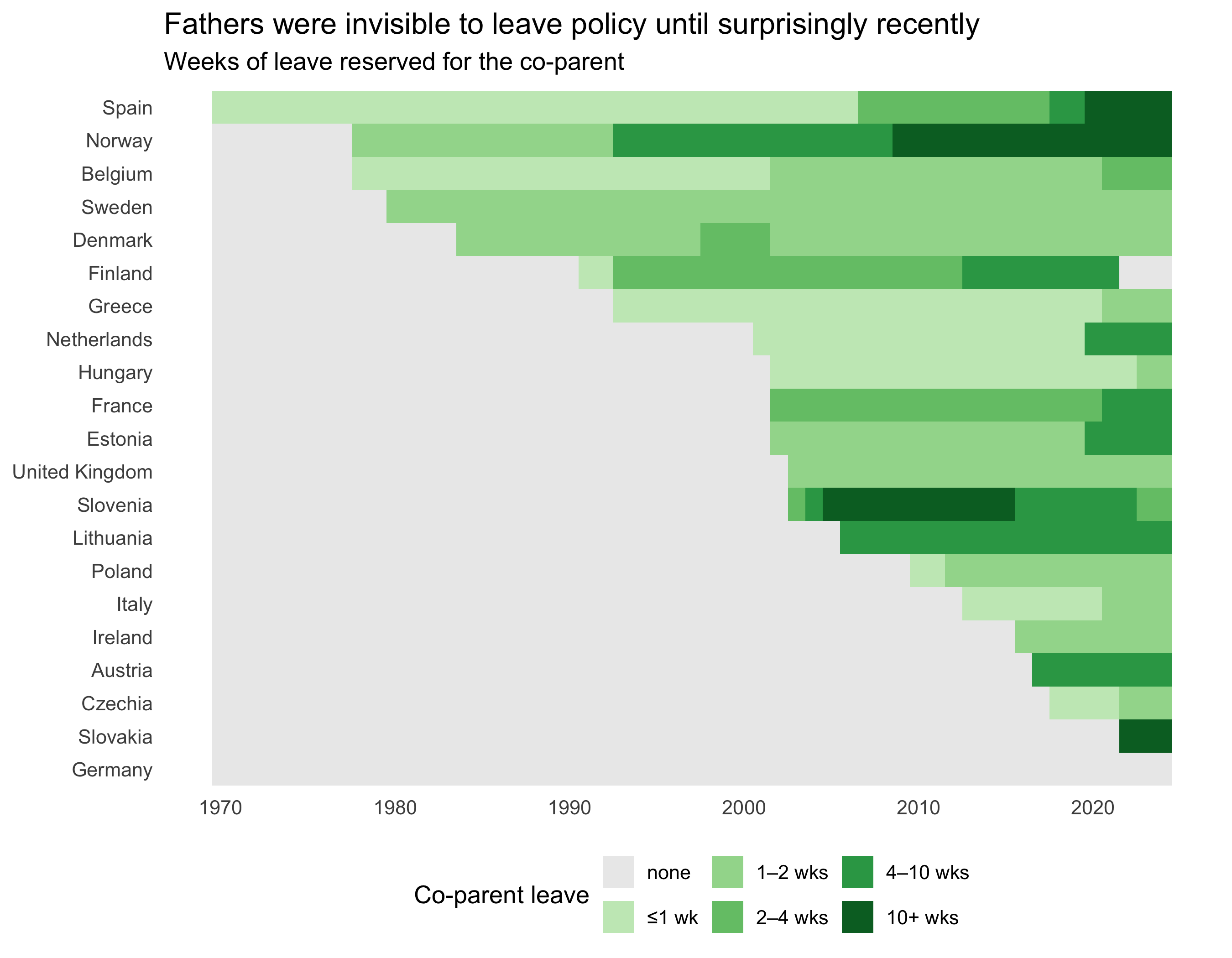
## The arrival of the co-parent
For most of the 20th century, "parenting leave" meant *maternity* leave.
The `co_ld` column — leave reserved for the co-parent (typically the father) —
lets us watch the second parent enter the policy frame.
```{r co-parent-tiles}
#| fig-height: 7
#| fig-cap: "Weeks of co-parent leave by country and year. Countries ordered by when they first granted any."
co <- eplp |>
  select(country_name, year, co_ld) |>
  mutate(co_ld = replace_na(co_ld, 0))

first_co <- co |>
  filter(co_ld > 0) |>
  summarise(first_year = min(year), .by = country_name)

co |>
  left_join(first_co, by = "country_name") |>
  mutate(
    country_name = fct_reorder(country_name, replace_na(first_year, 2030), .desc = TRUE),
    co_cat = cut(co_ld, breaks = c(-Inf, 0, 1, 2, 4, 10, Inf),
                 labels = c("none", "≤1 wk", "1–2 wks", "2–4 wks", "4–10 wks", "10+ wks"))
  ) |>
  ggplot(aes(year, country_name, fill = co_cat)) +
  geom_tile() +
  scale_fill_manual(
    values = c("grey92", "#c7e9c0", "#a1d99b", "#74c476", "#31a354", "#006d2c"),
    name = "Co-parent leave"
  ) +
  labs(
    title = "Fathers were invisible to leave policy until surprisingly recently",
    subtitle = "Weeks of leave reserved for the co-parent",
    x = NULL, y = NULL
  ) +
  theme(panel.grid = element_blank(), legend.position = "bottom")
```
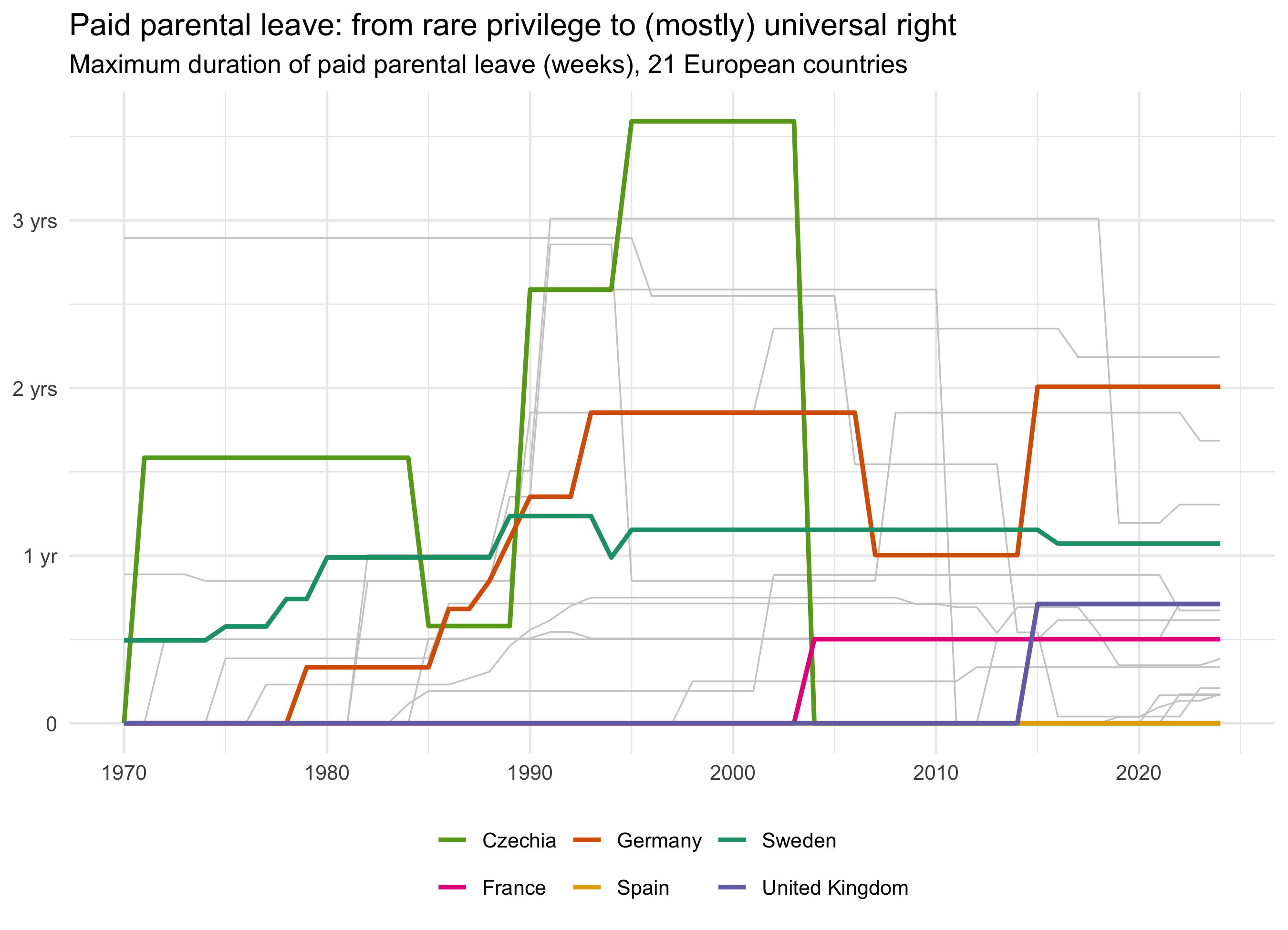
## How long can a parent stay home, paid?
`par1_ld` is the *longest possible* paid parental leave under each country's rules
(excluding maternity leave proper).
```{r paid-duration-spaghetti}
#| fig-height: 6.5
#| fig-cap: "Maximum paid parental leave duration. A handful of countries highlighted; all others in grey."
highlight <- c("Sweden", "Germany", "United Kingdom", "France", "Czechia", "Spain")

pal <- c("Sweden" = "#1b9e77", "Germany" = "#d95f02", "United Kingdom" = "#7570b3",
         "France" = "#e7298a", "Czechia" = "#66a61e", "Spain" = "#e6ab02")

p1 <- eplp |>
  select(country_name, year, par1_ld) |>
  mutate(par1_ld = replace_na(par1_ld, 0))

ggplot(p1, aes(year, par1_ld, group = country_name)) +
  geom_line(colour = "grey80", linewidth = 0.4) +
  geom_line(
    data = filter(p1, country_name %in% highlight),
    aes(colour = country_name), linewidth = 1.1
  ) +
  scale_colour_manual(values = pal, name = NULL) +
  scale_y_continuous(breaks = seq(0, 200, 52),
                     labels = c("0", "1 yr", "2 yrs", "3 yrs")) +
  labs(
    title = "Paid parental leave: from rare privilege to (mostly) universal right",
    subtitle = "Maximum duration of paid parental leave (weeks), 21 European countries",
    x = NULL, y = NULL
  ) +
  theme(legend.position = "bottom")
```
::: {.callout-warning}
## A measurement cliff, not a policy cliff
Czechia's paid parental leave appears to crash from ~3.6 years to zero in 2004. It didn't:
the Czech *rodičovský příspěvek* (parental allowance) continued — but from 2004 the dataset
reclassifies it out of the paid-parental-leave columns (the row carries a `user_note` flag),
while job-protected leave continues uninterrupted at 157 weeks. Harmonised policy datasets
are full of these definitional seams; the trick is to spot them before narrating them.
:::
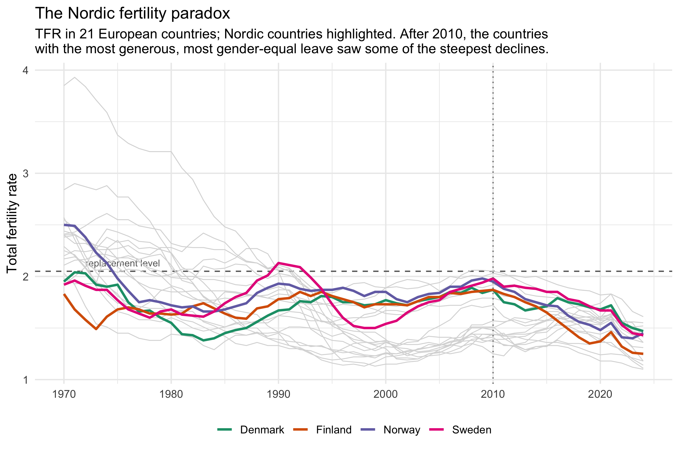
## Does any of this show up in the birth rate?
Parenting leave is now front-of-stage in the debate about **declining fertility in
high-income countries**. The argument, roughly: fertility is collapsing because having
children is too costly in time, money and careers — so make leave longer, better paid,
and more equally shared, and births should recover. Europe 1970–2024 is a decent natural
testing ground: 21 countries, wildly different policy paths, and (via the World Bank)
a complete total fertility rate (TFR) series for every country-year.
```{r tfr-join}
tfr <- read_csv("data/wb_tfr.csv", show_col_types = FALSE) |>
  mutate(country = if_else(iso2 == "GB", "UK", iso2))

# Total paid weeks available to a mother after birth:
# mandatory + voluntary maternity (post-birth) + longest paid parental scheme
leave <- eplp |>
  mutate(
    total_paid_mother = coalesce(mat_m_ld_ab, 0) + coalesce(mat_v_ld_ab, 0) +
      coalesce(par1_ld, 0)
  ) |>
  select(country, country_name, year, total_paid_mother, co_ld, par1_ld)

dat <- leave |> inner_join(tfr, by = c("country", "year"))
```
```{r tfr-trajectories}
#| fig-height: 6
#| fig-cap: "Total fertility rate, 1970–2024. The post-2010 slide is near-universal — including in the most generous leave regimes."
nordics <- c("Sweden", "Norway", "Finland", "Denmark")

dat |>
  mutate(group = if_else(country_name %in% nordics, country_name, "other")) |>
  ggplot(aes(year, tfr, group = country_name)) +
  geom_hline(yintercept = 2.05, linetype = "dashed", colour = "grey40") +
  annotate("text", x = 1972, y = 2.13, label = "replacement level",
           hjust = 0, size = 3.2, colour = "grey40") +
  geom_line(colour = "grey85", linewidth = 0.4) +
  geom_line(data = \(d) filter(d, group != "other"),
            aes(colour = group), linewidth = 1.1) +
  geom_vline(xintercept = 2010, linetype = "dotted", colour = "grey50") +
  scale_colour_brewer(palette = "Dark2", name = NULL) +
  labs(
    title = "The Nordic fertility paradox",
    subtitle = "TFR in 21 European countries; Nordic countries highlighted. After 2010, the countries\nwith the most generous, most gender-equal leave saw some of the steepest declines.",
    x = NULL, y = "Total fertility rate"
  ) +
  theme(legend.position = "bottom")
```
```{r decade-scatter}
#| fig-height: 4.5
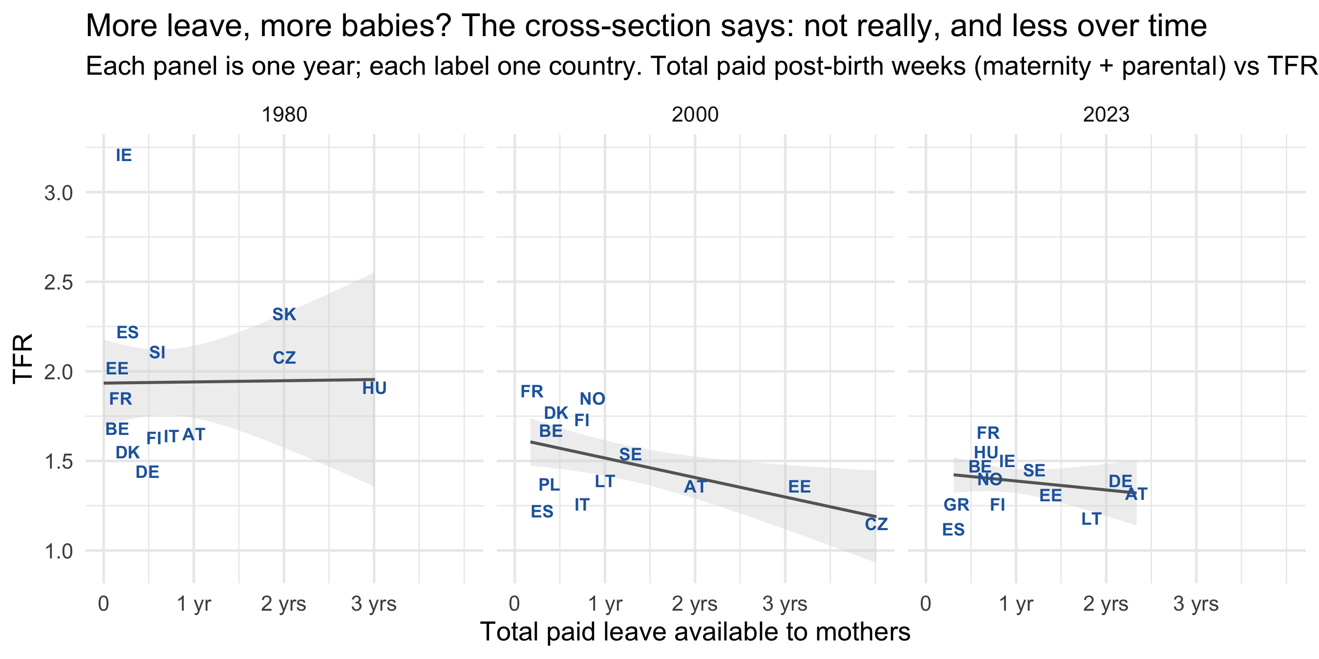
#| fig-cap: "Cross-sectional association between total paid leave available to mothers and TFR, by year."
dat |>
  filter(year %in% c(1980, 2000, 2023)) |>
  ggplot(aes(total_paid_mother, tfr)) +
  geom_smooth(method = "lm", se = TRUE, colour = "grey40",
              fill = "grey85", linewidth = 0.7) +
  geom_text(aes(label = country), size = 3, colour = "#2166ac",
            fontface = "bold", check_overlap = TRUE) +
  facet_wrap(~year) +
  scale_x_continuous(breaks = seq(0, 200, 52),
                     labels = c("0", "1 yr", "2 yrs", "3 yrs")) +
  labs(
    title = "More leave, more babies? The cross-section says: not really, and less over time",
    subtitle = "Each panel is one year; each label one country. Total paid post-birth weeks (maternity + parental) vs TFR.",
    x = "Total paid leave available to mothers", y = "TFR"
  )
```
```{r change-change}
#| fig-height: 6
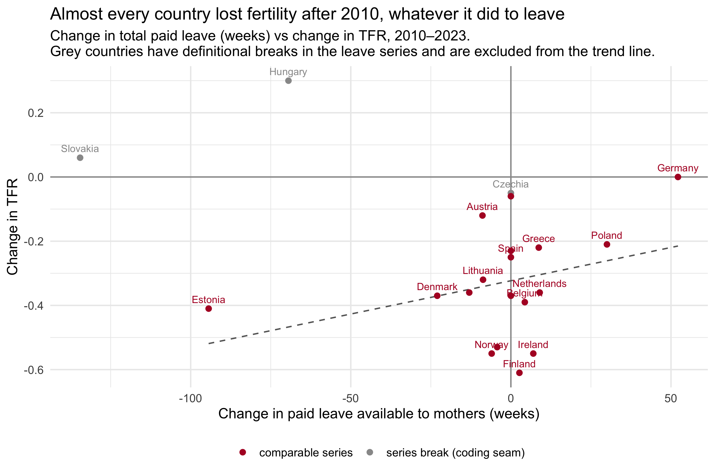
#| fig-cap: "Within-country changes, 2010 → 2023: did countries that expanded leave see smaller fertility declines?"
# CZ, SK and HU have definitional breaks in the paid-parental columns
# (allowances reclassified out of par1 while job protection continues),
# so their apparent leave "cuts" are coding seams, not reforms.
seams <- c("CZ", "SK", "HU")

chg <- dat |>
  filter(year %in% c(2010, 2023)) |>
  pivot_wider(id_cols = c(country, country_name),
              names_from = year,
              values_from = c(total_paid_mother, tfr)) |>
  mutate(
    d_leave = total_paid_mother_2023 - total_paid_mother_2010,
    d_tfr = tfr_2023 - tfr_2010,
    seam = country %in% seams
  )

ggplot(chg, aes(d_leave, d_tfr)) +
  geom_hline(yintercept = 0, colour = "grey60") +
  geom_vline(xintercept = 0, colour = "grey60") +
  geom_smooth(data = \(d) filter(d, !seam),
              method = "lm", se = FALSE, colour = "grey40",
              linetype = "dashed", linewidth = 0.6) +
  geom_point(aes(colour = seam), size = 2) +
  geom_text(aes(label = country_name, colour = seam), size = 3.2,
            vjust = -0.8, check_overlap = TRUE, show.legend = FALSE) +
  scale_colour_manual(
    values = c(`FALSE` = "#b2182b", `TRUE` = "grey60"),
    labels = c(`FALSE` = "comparable series", `TRUE` = "series break (coding seam)"),
    name = NULL
  ) +
  labs(
    title = "Almost every country lost fertility after 2010, whatever it did to leave",
    subtitle = "Change in total paid leave (weeks) vs change in TFR, 2010–2023.\nGrey countries have definitional breaks in the leave series and are excluded from the trend line.",
    x = "Change in paid leave available to mothers (weeks)",
    y = "Change in TFR"
  ) +
  theme(legend.position = "bottom")
```
### What this does and doesn't say
Three honest readings of these plots:
1. **No robust dose–response in sight.** The cross-section shows no positive
association (if anything the reverse, driven by long-leave/low-TFR Eastern Europe).
The within-country changes show a weakly positive slope that leans almost entirely
on Estonia — one influential point, not a pattern. Meanwhile the post-2010 decline
is remarkably synchronised across policy regimes —
which points to causes that don't vary much between European countries
(housing costs, labour-market precarity, partnership formation, norms around
intensive parenting, smartphones-and-dating, take your pick of the live hypotheses).
2. **This is not evidence leave "doesn't work".** Policy endogeneity runs hot here:
countries often expand family policy *because* fertility is falling (Hungary and
Poland's pronatalist turns are the loudest examples). That reverse causality biases
naive associations towards zero or below. Micro-level studies (e.g. of reform
discontinuities) are the right tool for causal claims; a country-year panel can
only frame the question.
3. **TFR is a tempo-distorted measure.** Period TFR drops when births are *postponed*,
even if completed family size is stable. Some of the post-2010 slide is timing;
how much is still an open fight in demography.