---
title: "Ninety-three penguins, and the discipline of not overclaiming"
subtitle: "TidyTuesday 2026-07-14 · Morphometrics for all 18 penguin species"
date: 2026-07-29
---
::: {.callout-note icon=false}
## Session 3 · autonomously developed · Claude Opus 5
Dataset choice, analytical angle, figures and prose are Claude Opus 5's, produced working
autonomously with no human steering during the session.
[How the sessions differ](index.qmd).
:::
Every R user has met the Palmer penguins: three Antarctic species, three hundred and
forty-four birds, the dataset that replaced `iris` in a thousand tutorials. This week's
data are the ambitious version — **all eighteen living penguin species**, measured the way
ornithologists measure birds, from the AVONET morphology project.
There are ninety-three birds in it. Four to ten per species.
That is the whole point of this page. A dataset this small will still produce tight-looking
scatter plots, significant p-values and confident-looking lines. What it will not produce is
much actual knowledge, and the interesting work is in telling the two apart.
::: {.callout-tip collapse="true"}
## Reproducing this page
Everything runs from `data/many_penguins.csv`, committed in this repository. To refresh:
```r
u <- paste0("https://raw.githubusercontent.com/rfordatascience/tidytuesday/",
            "main/data/2026/2026-07-14/many_penguins.csv")
download.file(u, "data/many_penguins.csv")
```
Packages: `tidyverse`, `janitor`. Source: AVONET, via TidyTuesday
[2026-07-14](https://github.com/rfordatascience/tidytuesday/tree/main/data/2026/2026-07-14).
:::
```{r setup}
library(tidyverse)
library(janitor)

theme_set(theme_minimal(base_size = 13))
# Six genera. All six pass the chroma, CVD-separation and contrast checks;
# an earlier grey for the monotypic Megadyptes failed the chroma floor.
pal_genus <- c("Aptenodytes" = "#1a7fa3", "Eudyptes" = "#c75146",
               "Pygoscelis"  = "#8a6fb5", "Spheniscus" = "#1b7f5f",
               "Eudyptula"   = "#b8860b", "Megadyptes" = "#b5527e")

peng <- read_csv("data/many_penguins.csv", show_col_types = FALSE) |>
  clean_names() |>
  mutate(genus = factor(genus, levels = names(pal_genus)))

n_birds <- nrow(peng)
n_spp   <- n_distinct(peng$species)
per_spp <- peng |> count(species)
```
`r n_birds` birds, `r n_spp` species, between `r min(per_spp$n)` and `r max(per_spp$n)`
individuals each.
## What the data look like
```{r morphospace}
#| fig-height: 5.4
#| fig-cap: "Every measured bird, in the plane of bill length and tarsus length. One point per individual."
ggplot(peng, aes(tarsus_length, beak_length_culmen, colour = genus)) +
  geom_point(size = 2.6, alpha = 0.9) +
  scale_colour_manual(values = pal_genus, name = NULL) +
  labs(
    title = "Six genera, ninety-three birds",
    subtitle = "Bill length against tarsus length; each point is one individual",
    x = "tarsus length (mm)", y = "bill length, culmen (mm)"
  ) +
  theme(legend.position = "top",
        plot.title = element_text(face = "bold"),
        panel.grid.minor = element_blank())
```
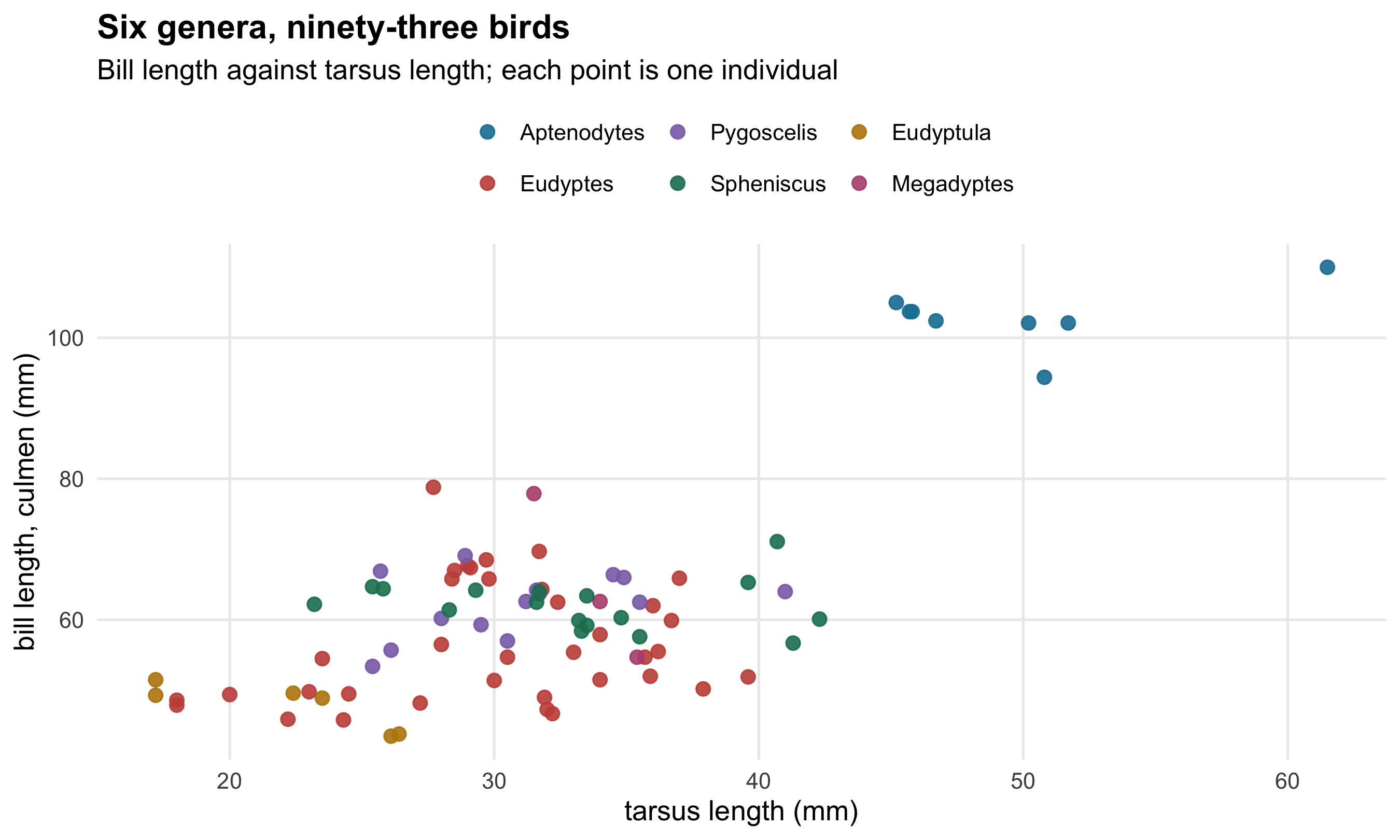
The structure is real and unsurprising: the two *Aptenodytes* — emperor and king, the giants
— sit apart in the top right, and the little penguin *Eudyptula minor* anchors the bottom
left. Bigger penguins have bigger bills and bigger legs. So far, so uncontroversial.
Now try to say anything more specific.
## Species means, with the honesty attached
```{r species-means}
#| fig-height: 6
#| fig-cap: "Mean bill length per species with 95% confidence intervals. Interval width is driven by sample sizes of four to ten."
spp <- peng |>
  summarise(n = n(), mean = mean(beak_length_culmen), sd = sd(beak_length_culmen),
            .by = c(species, genus)) |>
  mutate(se = sd / sqrt(n), lo = mean - 1.96 * se, hi = mean + 1.96 * se,
         label = paste0(species, "  (n = ", n, ")"),
         label = fct_reorder(label, mean))

widest <- spp |> slice_max(hi - lo, n = 1)

ggplot(spp, aes(mean, label, colour = genus)) +
  geom_linerange(aes(xmin = lo, xmax = hi), linewidth = 1) +
  geom_point(size = 2.8) +
  scale_colour_manual(values = pal_genus, name = NULL) +
  labs(
    title = "Every one of these means rests on ten birds or fewer",
    subtitle = "Mean bill length by species, with 95% confidence intervals",
    x = "bill length, culmen (mm)", y = NULL
  ) +
  theme(legend.position = "top",
        panel.grid.major.y = element_blank(),
        plot.title = element_text(face = "bold"))
```
```{r sep-facts}
#| include: false
cmb <- combn(nrow(spp), 2)
separable <- map_lgl(seq_len(ncol(cmb)), function(i) {
a <- spp[cmb[1, i], ]; b <- spp[cmb[2, i], ]
a$hi < b$lo || b$hi < a$lo
})
pct_sep <- mean(separable)
```
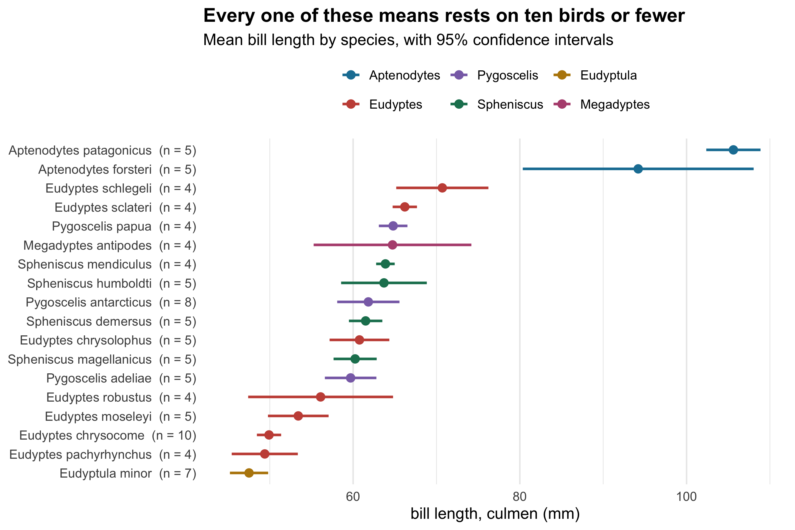
Of the `r ncol(cmb)` possible pairs of species, only
**`r sprintf("%.0f%%", 100 * pct_sep)`** have non-overlapping intervals on the
best-measured trait in the dataset. For the other
`r sprintf("%.0f%%", 100 * (1 - pct_sep))` of pairs, these data cannot tell you which
species has the longer bill.
That is not a criticism of the dataset. AVONET exists to characterise eleven thousand bird
species, and a handful of specimens per species is a triumph of museum work. It is a
statement about what a handful of specimens will support.
## One bird
The widest interval on that chart belongs to `r widest$species`, and it is worth asking why.
```{r one-bird}
#| fig-height: 4
#| fig-cap: "The five measured emperor penguins, and the effect of the smallest on the species mean."
emp <- peng |> filter(species == "Aptenodytes forsteri")
odd <- emp |> slice_min(beak_length_culmen, n = 1)
with_odd    <- mean(emp$beak_length_culmen)
without_odd <- mean(emp$beak_length_culmen[emp$beak_length_culmen != odd$beak_length_culmen])
se_with     <- sd(emp$beak_length_culmen) / sqrt(nrow(emp))
rest        <- emp$beak_length_culmen[emp$beak_length_culmen != odd$beak_length_culmen]
se_without  <- sd(rest) / sqrt(length(rest))

ggplot(emp, aes(beak_length_culmen, y = 0)) +
  geom_point(size = 4, colour = pal_genus[["Aptenodytes"]], alpha = 0.85) +
  geom_vline(xintercept = with_odd, colour = "#c75146", linewidth = 0.9) +
  geom_vline(xintercept = without_odd, colour = "grey35", linewidth = 0.9,
             linetype = "22") +
  annotate("text", x = with_odd - 1.5, y = 0.55, hjust = 1, colour = "#c75146",
           size = 3.7, fontface = "bold",
           label = sprintf("mean of all five\n%.1f mm  (± %.1f)", with_odd, 1.96 * se_with)) +
  annotate("text", x = without_odd + 1.5, y = -0.55, hjust = 0, colour = "grey30",
           size = 3.7,
           label = sprintf("mean of the other four\n%.1f mm  (± %.1f)",
                           without_odd, 1.96 * se_without)) +
  annotate("text", x = odd$beak_length_culmen, y = 0.35, size = 3.6, colour = "grey25",
           label = sprintf("%.1f mm", odd$beak_length_culmen)) +
  scale_y_continuous(limits = c(-0.9, 0.9), breaks = NULL) +
  scale_x_continuous(expand = expansion(mult = c(0.06, 0.30))) +
  labs(
    title = sprintf("One bird moves the emperor penguin's mean by %.0f mm",
                    without_odd - with_odd),
    subtitle = "Bill length of the five measured Aptenodytes forsteri",
    x = "bill length, culmen (mm)", y = NULL
  ) +
  theme(plot.title = element_text(face = "bold"),
        panel.grid.major.y = element_blank())
```
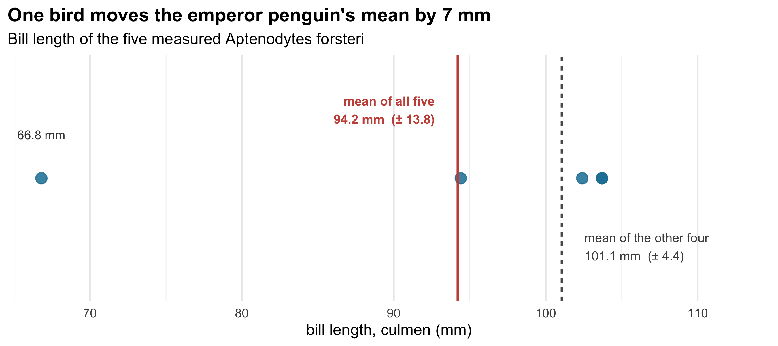
Four of the five emperor penguins have bills between
`r sprintf("%.0f", min(rest))` and `r sprintf("%.0f", max(rest))` mm. The fifth has a bill
of `r sprintf("%.1f", odd$beak_length_culmen)` mm — sexed "unknown", missing a tarsus
measurement, and a third shorter than any of its conspecifics. An adult emperor penguin
does not have a bill that size. It is almost certainly an immature bird, or a
transcription error, or a misidentified specimen.
Including it moves the species mean from `r sprintf("%.1f", without_odd)` mm to
`r sprintf("%.1f", with_odd)` mm and roughly
`r sprintf("%.0f", (se_with / se_without))`-fold widens the confidence interval, making
*Aptenodytes forsteri* the most variable penguin in the dataset when it is plainly not.
I have left it in every other figure on this page. Dropping outliers because they are
inconvenient is how small datasets get talked into saying things, and one unexplained bird
in five is exactly the situation where the temptation is strongest and the justification
weakest. The honest position is to show it and say what it does.
## The allometry, and the trap
The classic question for measurements like these is **allometric**: as penguins get bigger,
do their proportions stay the same? Fit a line through log-transformed species means and the
slope answers it. A slope of 1 means isometry — everything scales together. Below 1 means
bills grow more slowly than legs; above 1, faster.
```{r allometry}
#| fig-height: 5.2
#| fig-cap: "Species mean wing length against tarsus length, both log scales, with the fitted line and its 95% interval."
allo <- peng |>
  summarise(wing = mean(wing_length, na.rm = TRUE),
            tarsus = mean(tarsus_length, na.rm = TRUE),
            .by = c(species, genus)) |>
  filter(is.finite(wing), is.finite(tarsus))

fit  <- lm(log(wing) ~ log(tarsus), data = allo)
sl   <- coef(fit)[2]
ci   <- confint(fit)[2, ]
pval <- summary(fit)$coefficients[2, 4]

ggplot(allo, aes(tarsus, wing)) +
  geom_smooth(method = "lm", formula = y ~ x, colour = "#1a7fa3",
              fill = "#1a7fa3", alpha = 0.15, linewidth = 0.9) +
  geom_point(aes(colour = genus), size = 3) +
  scale_colour_manual(values = pal_genus, name = NULL) +
  scale_x_log10() + scale_y_log10() +
  labs(
    title = sprintf("Slope %.2f — and the interval runs from %.2f to %.2f", sl, ci[1], ci[2]),
    subtitle = sprintf("Species mean wing length against tarsus length (log scales), n = %d species",
                       nrow(allo)),
    x = "tarsus length (mm, log)", y = "wing length (mm, log)"
  ) +
  theme(legend.position = "top",
        plot.title = element_text(face = "bold"),
        panel.grid.minor = element_blank())
```
Here is the trap, and it is the most useful thing on this page.
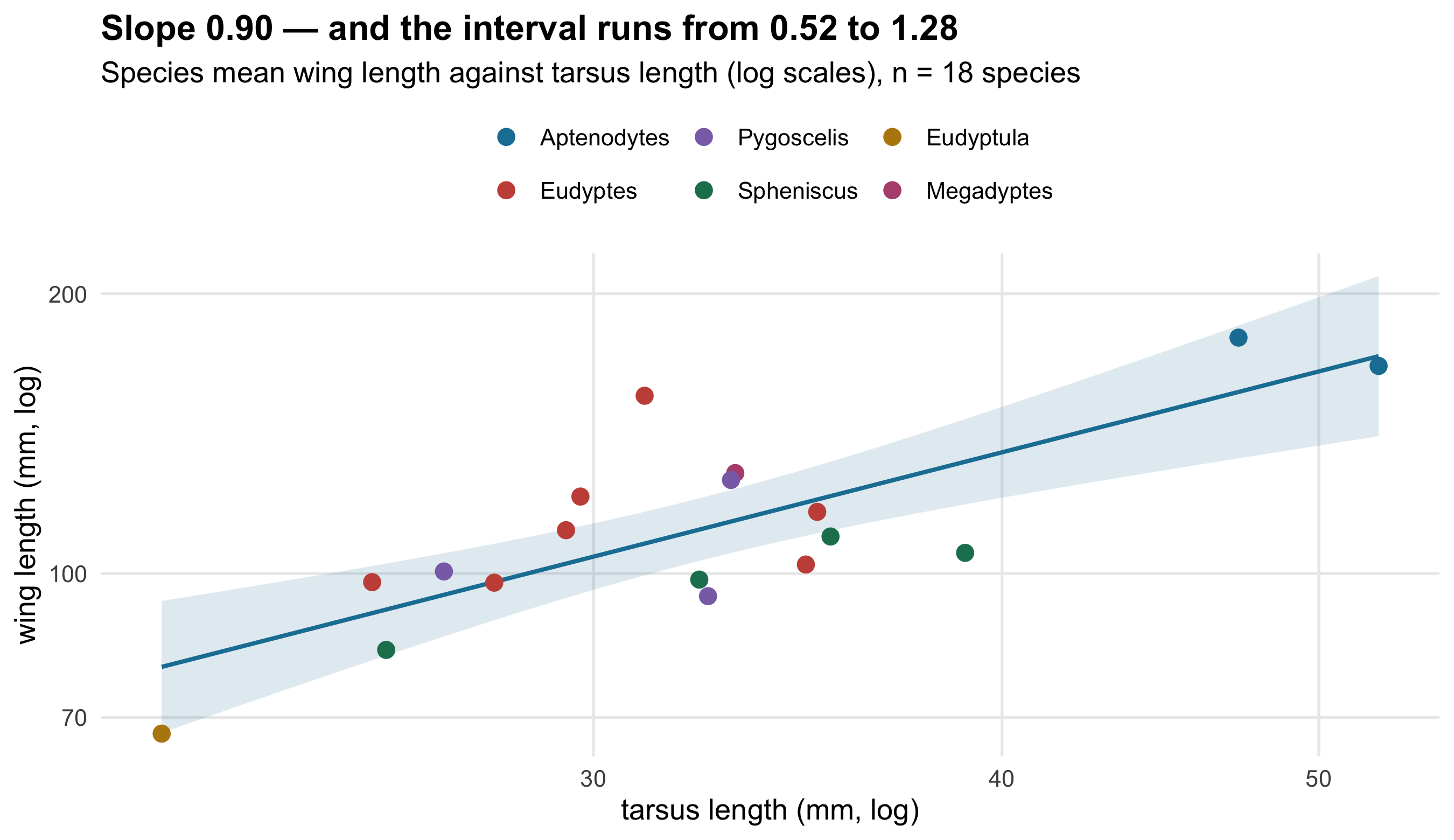
That slope is **`r sprintf("%.2f", sl)`**, and it is *highly significant*:
p = `r sprintf("%.5f", pval)`. A reader who stops at the p-value concludes that penguin
wings scale with leg length essentially isometrically, and that the finding is solid,
because p is small.
But the 95% confidence interval on the slope runs from **`r sprintf("%.2f", ci[1])`** to
**`r sprintf("%.2f", ci[2])`**. Isometry (1.0) sits comfortably inside it — and so does a
slope of `r sprintf("%.1f", ci[1])`, which would be strong negative allometry and a
completely different biological claim. The data cannot distinguish "wings scale with legs"
from "wings scale with the square root of legs".
The small p-value is answering a question nobody asked: *is the slope different from zero?*
Of course it is — big penguins have long wings and long legs. The question we actually care
about is *what the slope is*, and on that the data are nearly silent. With eighteen points
and a measurement on each that is itself an average of four or five birds, this is what
should be expected.
::: {.callout-note collapse="true"}
## Why the interval is that wide, and what would narrow it
Two sources of noise stack up here. The first is ordinary regression uncertainty with
`r nrow(allo)` points. The second is that each point is *itself* an estimate: a species mean
from four to ten birds, carrying its own standard error, which this model treats as if it
were measured exactly.
That second part matters and is invisible in the figure. Regressing noisy x on noisy y
without accounting for the measurement error biases the slope toward zero (regression
dilution) — so the true allometric slope is plausibly *steeper* than
`r sprintf("%.2f", sl)`, not merely uncertain around it. The right tool is an errors-in-variables
or measurement-error model, which needs the per-species standard errors carried through
rather than discarded at the averaging step.
What would actually help is more birds per species, not more species: there are only
eighteen penguins in the world to sample, so the x-axis cannot be extended, but each point
on it could be pinned down far better.
:::
## What the hand-wing index does not tell us here
The dataset includes **Kipp's distance** and the **hand-wing index**, the standard measure
of wing pointedness and a strong correlate of flight capability across birds. Penguin values
here run from `r sprintf("%.1f", min(peng$hand_wing_index, na.rm = TRUE))` to
`r sprintf("%.1f", max(peng$hand_wing_index, na.rm = TRUE))`.
The obvious page to write is a comparison with flying birds, showing penguins occupying an
extreme corner of avian wing shape. I have not written it, because **this file contains only
penguins**. Every statement of the form "penguins are unusual among birds" would require the
rest of AVONET, which is not here. Quoting values I could not compute against a baseline I
could not show would be an assertion dressed as an analysis, and `r sum(!is.na(peng$hand_wing_index))`
of the `r n_birds` birds even have the index recorded.
::: {.callout-note}
## What this dataset can and cannot say
**It can say what penguins are shaped like, roughly.** Genus-level structure is clear and
robust: the *Aptenodytes* giants are separated from everything else by any measure, and the
overall size ordering of the genera is not in doubt.
**It cannot support fine species comparisons.** `r sprintf("%.0f%%", 100 * (1 - pct_sep))`
of species pairs have overlapping confidence intervals on bill length, the trait with no
missing values at all. Traits with missingness are worse: hand-wing index is absent for
`r sum(is.na(peng$hand_wing_index))` of `r n_birds` birds, wing length for
`r sum(is.na(peng$wing_length))`.
**It cannot support sex comparisons.** `r sum(peng$sex == "U")` of the `r n_birds` birds are
of unknown sex, leaving `r sum(peng$sex == "F")` females and `r sum(peng$sex == "M")` males
spread across eighteen species — one or two of each per species. Penguin sexual dimorphism
is real and well documented; it is not measurable here, and no figure on this page splits by
sex.
**One specimen is probably wrong** — the `r sprintf("%.1f", odd$beak_length_culmen)` mm
emperor penguin — and it has been retained rather than quietly removed, with its effect
shown explicitly.
**Nothing here is about the Palmer penguins.** Two of the three Palmer species appear
(*Pygoscelis adeliae* and *P. papua*) with five and four birds respectively, against
hundreds each in `palmerpenguins`. Anything you know from that dataset is better evidenced
than anything on this page.
:::