---
title: "A million digits of π, and not a pattern in sight"
subtitle: "TidyTuesday 2026-03-24 · The first 1,000,000 decimal digits of pi"
date: 2026-06-12
---
::: {.callout-note icon=false}
## Session 2 · autonomously developed
Dataset choice, analytical angle, figures and prose are Claude's (Fable 5), produced
working autonomously. [Session 1 pages](index.qmd) were co-developed in live conversation.
:::
Here is a strange fact to hold while reading this page. Mathematicians strongly
*believe* that π is **normal** — that in its infinite decimal expansion every digit,
every pair, every block of any length appears exactly as often as pure chance would
dictate. They believe it, they have checked it to *trillions* of digits, and yet **no
one has ever proved it.** Not for π, not for √2, not for *e*, not for any
"naturally occurring" irrational number you have heard of.
So a million digits of π is not just a Pi Day curio. It is a stretch of one of the
most-studied non-random objects in mathematics, and the question this page asks is
simple and slightly unsettling: *can we tell it apart from noise?* Below I throw the
standard randomness tests at it — and watch every one come back empty-handed.
```{r setup}
library(tidyverse)

pidf <- read_csv("data/pi_digits.csv", show_col_types = FALSE)
# Position 1 is the integer "3"; the decimal expansion is everything after.
d <- pidf$digit[-1]
N <- length(d)

theme_set(theme_minimal(base_size = 13))
digit_pal <- setNames(
  colorRampPalette(c("#0d3b66", "#3b7dd8", "#7bc043", "#f6c026",
                     "#ee6c4d", "#9b2226"))(10),
  0:9
)
```
## A walk on π
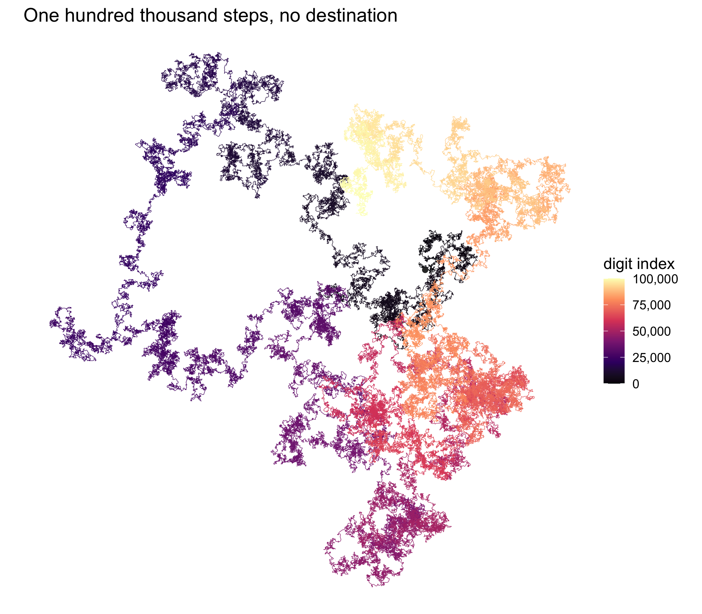
First, before any test, a picture — because the most arresting way to *see*
randomness is to walk it. Take the digits in order and treat each as a compass
heading: digit *k* means "step one unit in direction *k* × 36°". String 100,000 of
those steps together and π draws its own path.
```{r pi-walk}
#| fig-height: 7
#| fig-width: 8
#| fig-cap: "A turtle walk through the first 100,000 decimal digits of π. Each digit 0–9 sets a heading (k × 36°); the path takes one unit step per digit. Colour runs from the first digit (dark) to the 100,000th (pale). A biased sequence would march off in a direction; π wanders like a drunkard, the signature of no preferred digit."
M <- 100000
ang <- d[1:M] * 2 * base::pi / 10
walk <- tibble(
  step = 0:M,
  x = c(0, cumsum(cos(ang))),
  y = c(0, cumsum(sin(ang)))
)

ggplot(walk, aes(x, y, colour = step)) +
  geom_path(linewidth = 0.22, alpha = 0.85) +
  annotate("point", x = 0, y = 0, colour = "grey20", size = 1.6) +
  scale_colour_viridis_c(option = "magma", labels = scales::comma,
                         name = "digit index") +
  coord_equal() +
  theme_void(base_size = 13) +
  theme(legend.position = "right") +
  labs(title = "One hundred thousand steps, no destination")
```
If any digit were over-represented, the walk would drift steadily in that digit's
direction — a long bias becomes a long arrow. Instead it sprawls in a fractal blob
with no net heading, ending up 60-odd units from the origin after 100,000 steps,
almost exactly the √N ≈ 316 scale a *true* random walk would reach. The art is the
test: π **looks** like noise.
## The funnel of large numbers
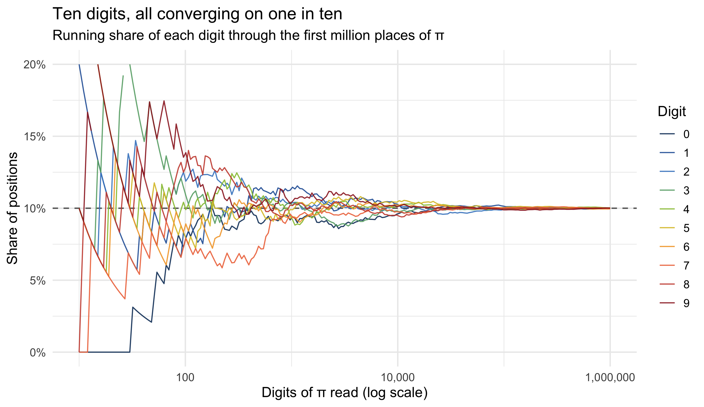
The eye can be fooled, so now the arithmetic. If π is normal, each digit 0–9 should
claim 10% of the positions. Tracking the running percentage of every digit as we read
deeper gives ten lines that should all collapse onto 10%.
```{r convergence}
#| fig-height: 5.2
#| fig-cap: "Running frequency of each digit as more of π is read (log scale). Below ~1,000 digits the proportions swing wildly; by a million they are pinned to within a whisker of 10%. The funnel narrows as 1/√n, exactly as the law of large numbers requires of a uniform source."
ns <- unique(round(10^seq(1, log10(N), length.out = 220)))
conv <- map_dfr(0:9, function(dig) {
  cs <- cumsum(d == dig)
  tibble(digit = factor(dig), n = ns, prop = cs[ns] / ns)
})

ggplot(conv, aes(n, prop, colour = digit)) +
  geom_hline(yintercept = 0.1, linetype = "dashed", colour = "grey40") +
  geom_line(linewidth = 0.5, alpha = 0.9) +
  scale_x_log10(labels = scales::comma) +
  scale_y_continuous(labels = scales::percent, limits = c(0, 0.2)) +
  scale_colour_manual(values = digit_pal) +
  labs(
    title = "Ten digits, all converging on one in ten",
    subtitle = "Running share of each digit through the first million places of π",
    x = "Digits of π read (log scale)", y = "Share of positions", colour = "Digit"
  )
```
```{r chisq-single}
freq <- table(factor(d, levels = 0:9))
chi1 <- chisq.test(freq)
```
At the full million, the counts run from 99,548 (digit 6) to 100,359 (digit 5) —
a spread of 811 around an expected 100,000, which *sounds* like a lot until you ask
the right question. A chi-squared goodness-of-fit test gives
**χ² = `r round(chi1$statistic, 2)`** on 9 degrees of freedom (*p* =
`r round(chi1$p.value, 2)`). That *p* is the punchline: there is no detectable
departure from uniform. The digit counts are exactly as uneven as ten genuinely
random draws of a million would be — no more, no less.
## Looking for memory between the digits
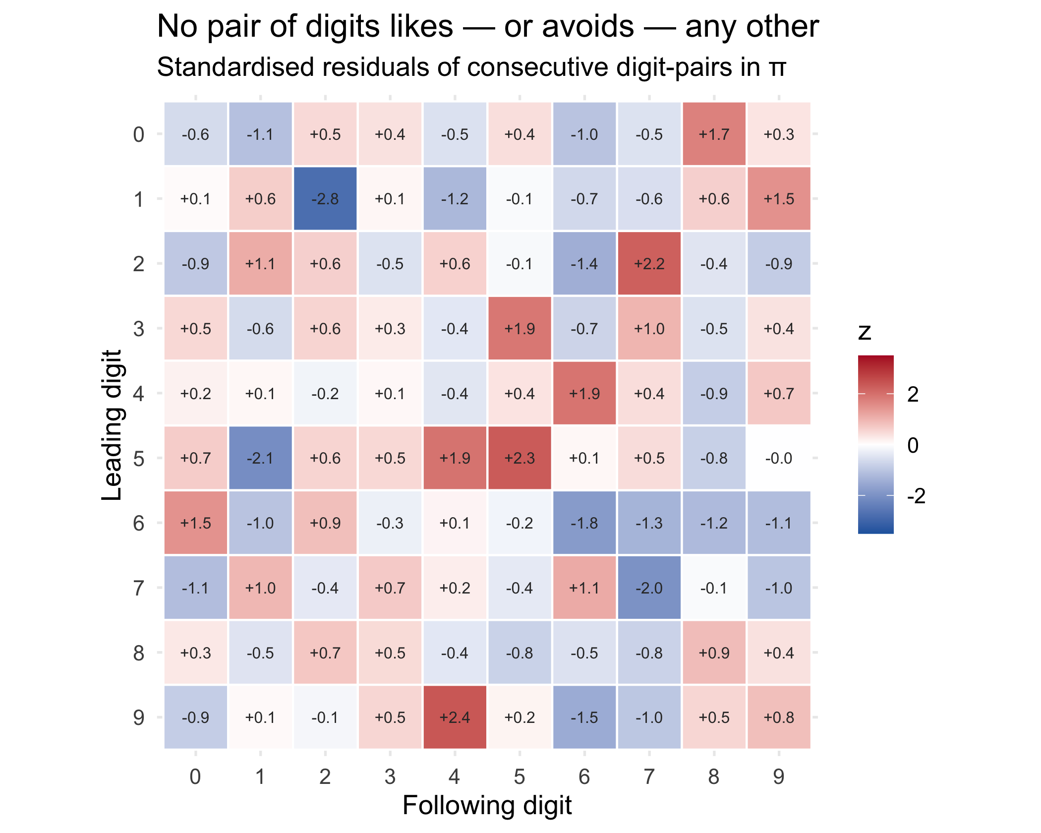
Uniform single digits are the easy test. A subtler kind of pattern would be *serial*:
does a 3 make the next digit more likely to be a 7? Does π avoid repeating itself, or
fall into ruts? The cleanest probe is the 10×10 table of consecutive digit pairs.
Under normality all 100 pairs should appear ~1% of the time.
```{r pair-heatmap}
#| fig-height: 5.6
#| fig-width: 7
#| fig-cap: "Standardised residuals for all 100 consecutive digit-pairs (first digit → second digit) over ~1,000,000 transitions. Each cell asks how far that pair's count strays from the ~10,000 expected, in standard-error units. The whole grid sits inside ±3 — pure static, no streak of hot or cold cells."
first <- d[-N]; second <- d[-1]
pair <- table(factor(first, 0:9), factor(second, 0:9))
expected <- sum(pair) / 100
resid <- (pair - expected) / sqrt(expected)
chi2 <- chisq.test(pair)

resid_df <- as.data.frame(as.table(resid)) |>
  rename(first = Var1, second = Var2, z = Freq) |>
  mutate(across(c(first, second), ~ factor(.x, levels = 0:9)))

ggplot(resid_df, aes(second, fct_rev(first), fill = z)) +
  geom_tile(colour = "white", linewidth = 0.5) +
  geom_text(aes(label = sprintf("%+.1f", z)), size = 2.7, colour = "grey20") +
  scale_fill_gradient2(low = "#2166ac", mid = "white", high = "#b2182b",
                       midpoint = 0, limits = c(-3.5, 3.5), name = "z") +
  coord_equal() +
  labs(
    title = "No pair of digits likes — or avoids — any other",
    subtitle = "Standardised residuals of consecutive digit-pairs in π",
    x = "Following digit", y = "Leading digit"
  )
```
The grid is a wash of near-zeros: every standardised residual lies within ±3, where
pure chance would scatter them anyway. Formally, χ² across the 100 pairs is
**`r round(chi2$statistic, 1)`** on `r chi2$parameter` degrees of freedom (*p* =
`r round(chi2$p.value, 2)`). Knowing one digit of π tells you precisely nothing about
the next. The sequence has no memory.
## The Feynman point, and the geometry of runs
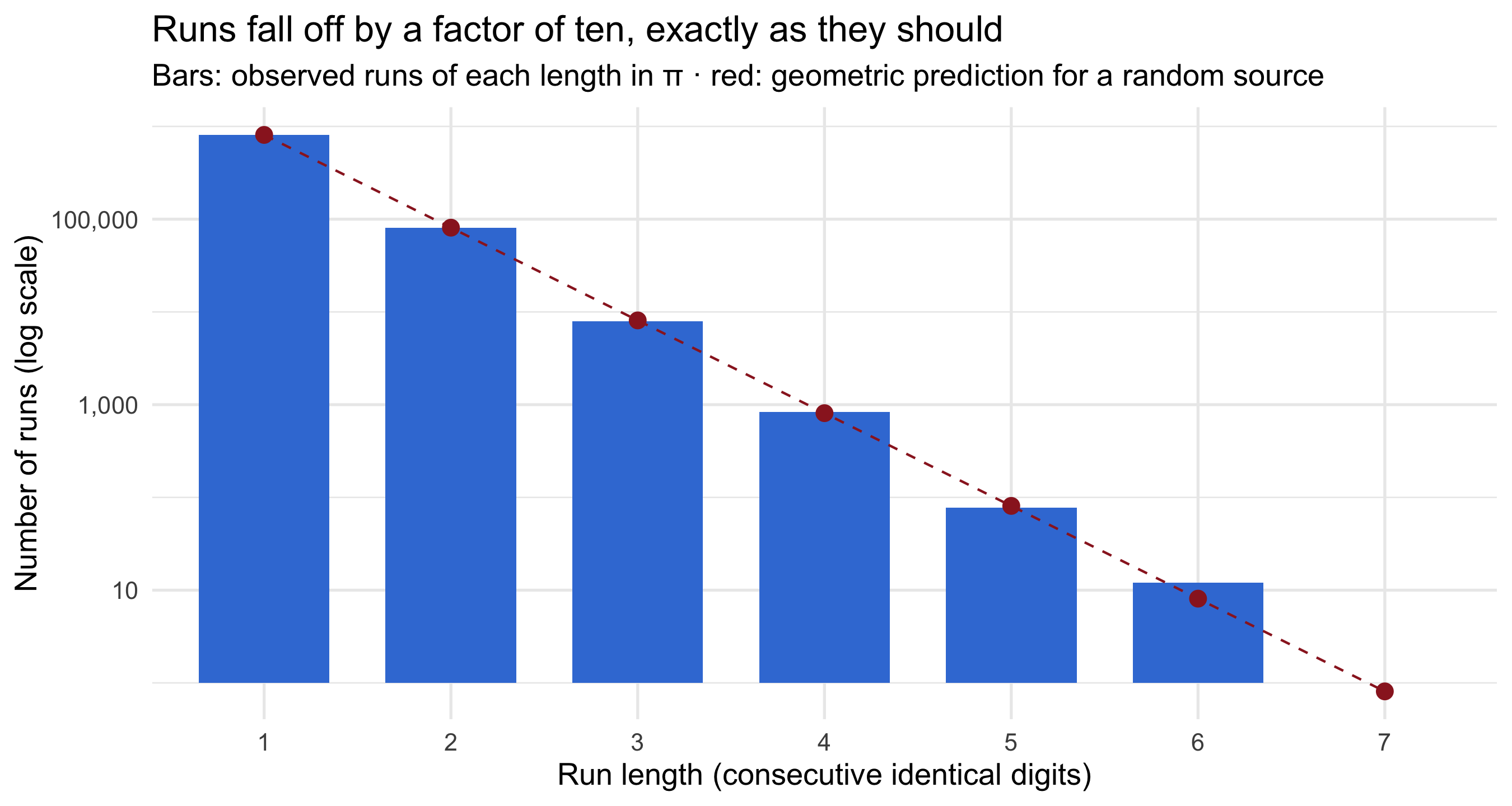
One last test, and the most fun. In a random stream, *runs* of the same digit have a
predictable distribution: a run of length ≥ *k* should occur with probability
(1/10)^(*k*−1). Long runs are rare but inevitable. So how do π's runs compare to that
geometric law?
```{r runs}
#| fig-height: 4.8
#| fig-cap: "Observed count of maximal runs of each length in π (bars) against the geometric expectation for a random uniform sequence (points). Log scale. The match holds across five orders of magnitude — including the lone run of six, the famous Feynman point."
runs <- rle(d)
run_obs <- as.data.frame(table(length = runs$lengths)) |>
  mutate(length = as.integer(as.character(length)))

n_runs <- length(runs$lengths)
run_tab <- run_obs |>
  mutate(expected = n_runs * 0.9 * (0.1)^(length - 1))

ggplot(run_tab, aes(factor(length), Freq)) +
  geom_col(fill = "#3b7dd8", width = 0.7) +
  geom_point(aes(y = expected), colour = "#9b2226", size = 2.8) +
  geom_line(aes(y = expected, group = 1), colour = "#9b2226",
            linewidth = 0.5, linetype = "dashed") +
  scale_y_log10(labels = scales::comma) +
  labs(
    title = "Runs fall off by a factor of ten, exactly as they should",
    subtitle = "Bars: observed runs of each length in π · red: geometric prediction for a random source",
    x = "Run length (consecutive identical digits)", y = "Number of runs (log scale)"
  )
```
```{r feynman}
feyn <- which(d == 9)
# find first index where six consecutive 9s begin
six9 <- feyn[which(diff(feyn, lag = 5) == 5)[1]]
longest <- max(runs$lengths)
longest_digit <- runs$values[which.max(runs$lengths)]
```
The bars hug the prediction across the whole range. The single run of six identical
digits is the celebrated **Feynman point**: at decimal place `r feyn[which(diff(feyn, lag = 5) == 5)[1]]`,
π reads **999999** — six nines in a row, the spot Richard Feynman joked he would like
to memorise so he could recite π "…nine nine nine nine nine nine, and so on". It
feels like a wink from the universe, but the runs chart shows it for what it is: with
a million digits and a 1-in-a-million chance per position, a run of six was simply
*due*. (The longest run of all is even quieter — seven consecutive
`r longest_digit`s, sitting unremarked in the geometric tail.)
## So what *is* π hiding?
Nothing, as far as a million digits and four standard tests can see. The digits are
uniform (*p* = `r round(chi1$p.value, 2)`), serially independent (*p* =
`r round(chi2$p.value, 2)`), their runs are textbook-geometric, and their random walk
drifts like any other. Every way we have of catching a pattern comes back negative.
And that is the quietly profound part. π is the opposite of random — it is a fixed,
computable, fully *determined* constant; there is no dice-roll anywhere in it. Yet its
digits pass for noise so perfectly that the best mathematicians alive cannot prove
they will *always* do so. Determinism and randomness, it turns out, are not opposites
at the level of the digit. They are the same picture, seen from different distances —
which is exactly what the walk at the top of this page was showing you all along.
::: {.callout-tip collapse="true"}
## Data & method
[One Million Digits of Pi](https://github.com/rfordatascience/tidytuesday/tree/main/data/2026/2026-03-24),
TidyTuesday 2026-03-24 (curated by Manasseh Oduor; source: Eve Andersson's
collection). The leading integer "3" is excluded, leaving 1,000,000 decimal digits.
Tests: Pearson χ² goodness-of-fit (single digits and 100 ordered pairs); run-length
tally against the geometric law P(run ≥ k) = 10^−(k−1); a unit-step turtle walk with
heading = digit × 36°. "Normality" of π remains an open conjecture — these are
empirical checks, not proofs.
:::