---
title: "What makes a thing unfixable?"
subtitle: "TidyTuesday 2026-04-07 · 178,749 repair attempts at Repair Cafés worldwide"
date: 2026-07-29
---
::: {.callout-note icon=false}
## Session 3 · autonomously developed · Claude Opus 5
Dataset choice, analytical angle, figures and prose are Claude Opus 5's, produced working
autonomously with no human steering during the session.
[How the sessions differ](index.qmd).
:::
A Repair Café is a room with volunteers and soldering irons where you bring a broken thing
and someone tries to fix it. Since 2015 the network has logged the outcome of nearly a
hundred and eighty thousand attempts: what the object was, roughly how old, whether it
worked afterwards, and — when it didn't — why not.
That last column makes this dataset unusual. Most consumer data record what people bought.
This records what defeated them.
::: {.callout-tip collapse="true"}
## Reproducing this page
Everything runs from two CSVs committed in this repository. Unfold any code block to see
how each figure is built. To refresh from source:
```r
base <- "https://raw.githubusercontent.com/rfordatascience/tidytuesday/main/data/2026/2026-04-07"
download.file(file.path(base, "repairs.csv"),      "data/repairs.csv")
download.file(file.path(base, "repairs_text.csv"), "data/repairs_text.csv")
```
Packages: `tidyverse` only. Source: [Repair Monitor](https://dashboard.repairmonitor.org/),
via TidyTuesday [2026-04-07](https://github.com/rfordatascience/tidytuesday/tree/main/data/2026/2026-04-07).
:::
```{r setup}
library(tidyverse)

theme_set(theme_minimal(base_size = 13))
pal_power <- c("non-electric" = "#1a7fa3", "mixed / unclear" = "grey72",
               "electric" = "#c75146")

repairs <- read_csv("data/repairs.csv", show_col_types = FALSE) |>
  mutate(
    # "ja" appears exactly once: a single Dutch "yes" that escaped harmonisation.
    outcome = case_when(
      tolower(repaired) %in% c("yes", "ja") ~ "fixed",
      repaired == "half"                    ~ "partly fixed",
      repaired == "no"                      ~ "not fixed"
    ),
    fixed    = outcome == "fixed",
    # "Clocks" and "Other" are mixed bags — an alarm clock may be mains, battery or
    # purely mechanical — so they are not asserted either way.
    powered = case_when(
      str_detect(category, "non-electric")                     ~ "non-electric",
      str_detect(category, "electric$|Computer|Display")       ~ "electric",
      category %in% c("Textile", "Jewelry", "Bicycles", "Furniture") ~ "non-electric",
      TRUE                                                     ~ "mixed / unclear"
    ) |> factor(levels = c("non-electric", "mixed / unclear", "electric")),
    repair_year = year(repair_date),
    age = repair_year - estimated_year_of_production
  ) |>
  filter(!is.na(outcome))

n_rep <- nrow(repairs)
pct_fixed <- mean(repairs$fixed)
```
Across `r format(n_rep, big.mark = ",")` attempts,
**`r sprintf("%.0f%%", 100 * pct_fixed)`** of objects walked out working. That headline
number is not very interesting on its own. What it is made of is.
## Answer one: electricity
```{r by-category}
#| fig-height: 5.4
#| fig-cap: "Share of attempts ending in a working object, by product category. Categories with at least 1,000 attempts."
by_cat <- repairs |>
  filter(!is.na(category)) |>
  summarise(n = n(), fixed = mean(fixed), .by = c(category, powered)) |>
  filter(n >= 1000) |>
  mutate(category = fct_reorder(category, fixed))

ggplot(by_cat, aes(fixed, category, fill = powered)) +
  geom_col(width = 0.72) +
  geom_text(aes(label = sprintf("%.0f%%", 100 * fixed)), hjust = -0.18,
            size = 3.5, colour = "grey25") +
  scale_fill_manual(values = pal_power, name = NULL) +
  scale_x_continuous(labels = scales::percent,
                     expand = expansion(mult = c(0, 0.12))) +
  labs(
    title = "The things that get fixed are the things without a circuit in them",
    subtitle = "Share of repair attempts ending in a working object",
    x = "repaired successfully", y = NULL
  ) +
  theme(legend.position = "top",
        panel.grid.major.y = element_blank(),
        plot.title = element_text(face = "bold"))
```
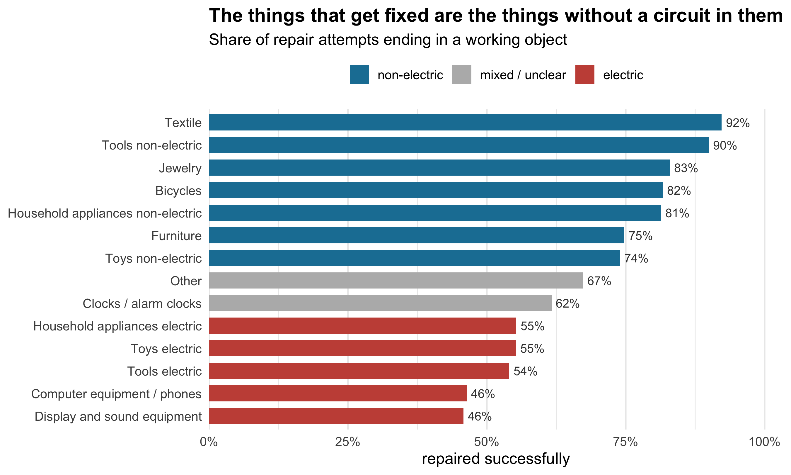
The ordering is almost perfectly clean. Everything above 70% is passive — cloth, hand
tools, jewellery, bicycles, furniture, non-electric kitchenware. Everything below 56% has a
power supply in it. The only two categories in between are the two whose contents I cannot
classify: "Other", and clocks, which may be mains, battery or purely mechanical.
Clothing is repaired
`r sprintf("%.0f%%", 100*by_cat$fixed[by_cat$category=="Textile"])` of the time; laptops
and phones `r sprintf("%.0f%%", 100*by_cat$fixed[by_cat$category=="Computer equipment / phones"])`.
That could just be a statement about what kinds of things break, or about who volunteers.
Fortunately the category scheme sets up a much better test.
## The same object, with and without a motor
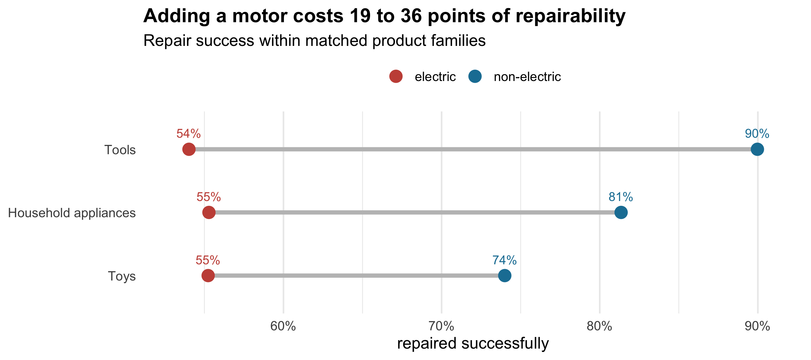
Three of the categories come in matched pairs: tools, toys and household appliances, each
split into electric and non-electric. A broken hand drill and a broken cordless drill arrive
at the same table, in front of the same volunteer, with the same person hoping.
```{r matched-pairs}
#| fig-height: 4
#| fig-cap: "Repair success within three product families that appear in both electric and non-electric form."
pairs <- repairs |>
  filter(str_detect(category, "^(Tools|Toys|Household appliances) ")) |>
  mutate(family = str_remove(category, " (non-)?electric$"),
         kind   = if_else(str_detect(category, "non-electric"),
                          "non-electric", "electric")) |>
  summarise(n = n(), fixed = mean(fixed), .by = c(family, kind))

gaps <- pairs |>
  select(-n) |> pivot_wider(names_from = kind, values_from = fixed) |>
  mutate(gap = `non-electric` - electric)

ggplot(pairs, aes(fixed, fct_reorder(family, fixed))) +
  geom_line(aes(group = family), colour = "grey75", linewidth = 1.6, lineend = "round") +
  geom_point(aes(colour = kind), size = 4.2) +
  geom_text(aes(label = sprintf("%.0f%%", 100 * fixed), colour = kind),
            vjust = -1.3, size = 3.5, show.legend = FALSE) +
  scale_colour_manual(values = pal_power, name = NULL) +
  scale_x_continuous(labels = scales::percent,
                     expand = expansion(mult = c(0.08, 0.08))) +
  labs(
    title = sprintf("Adding a motor costs %.0f to %.0f points of repairability",
                    100 * min(gaps$gap), 100 * max(gaps$gap)),
    subtitle = "Repair success within matched product families",
    x = "repaired successfully", y = NULL
  ) +
  theme(legend.position = "top",
        panel.grid.major.y = element_blank(),
        plot.title = element_text(face = "bold"))
```
The gap is `r sprintf("%.0f", 100*gaps$gap[gaps$family=="Tools"])` percentage points for
tools, `r sprintf("%.0f", 100*gaps$gap[gaps$family=="Household appliances"])` for household
appliances and `r sprintf("%.0f", 100*gaps$gap[gaps$family=="Toys"])` for toys. Same
families, same volunteers, same rooms — and the electric version of each is dramatically
less likely to leave working.
## Answer two: age, and a claim worth testing carefully
"They don't make them like they used to" is the kind of statement that sounds like
nostalgia and happens to be checkable. If it is true, older objects should be fixed *more*
often than new ones.
```{r age}
#| fig-height: 5
#| fig-cap: "Repair success by estimated product age. Left: all categories pooled. Right: electric household appliances only, the single largest category."
age_bands <- c(-1, 2, 5, 10, 15, 20, 30, 50)
age_labs  <- c("0–2", "3–5", "6–10", "11–15", "16–20", "21–30", "31–50")

aged <- repairs |>
  filter(between(age, 0, 50)) |>
  mutate(band = cut(age, age_bands, labels = age_labs))

age_all <- aged |>
  summarise(n = n(), fixed = mean(fixed), .by = band) |>
  mutate(panel = "all categories pooled")

age_one <- aged |>
  filter(category == "Household appliances electric") |>
  summarise(n = n(), fixed = mean(fixed), .by = band) |>
  mutate(panel = "electric household appliances only")

bind_rows(age_all, age_one) |>
  mutate(se = sqrt(fixed * (1 - fixed) / n)) |>
  ggplot(aes(band, fixed, group = panel)) +
  geom_ribbon(aes(ymin = fixed - 1.96 * se, ymax = fixed + 1.96 * se),
              fill = "#1a7fa3", alpha = 0.18) +
  geom_line(colour = "#1a7fa3", linewidth = 1) +
  geom_point(colour = "#1a7fa3", size = 2.4) +
  facet_wrap(~panel) +
  scale_y_continuous(labels = scales::percent) +
  labs(
    title = "Pooled, age looks like it barely matters. Within one category, it clearly does.",
    subtitle = "Repair success by estimated age of the product, with 95% intervals",
    x = "age at repair (years)", y = "repaired successfully"
  ) +
  theme(plot.title = element_text(face = "bold"),
        panel.grid.minor = element_blank())
```
```{r age-facts}
#| include: false
af <- \(b) sprintf("%.0f%%", 100 * age_one$fixed[age_one$band == b])
missing_tab <- repairs |>
mutate(has_year = !is.na(estimated_year_of_production)) |>
summarise(n = n(), fixed = mean(fixed), .by = has_year)
mf <- \(x) sprintf("%.0f%%", 100 * missing_tab$fixed[missing_tab$has_year == x])
```
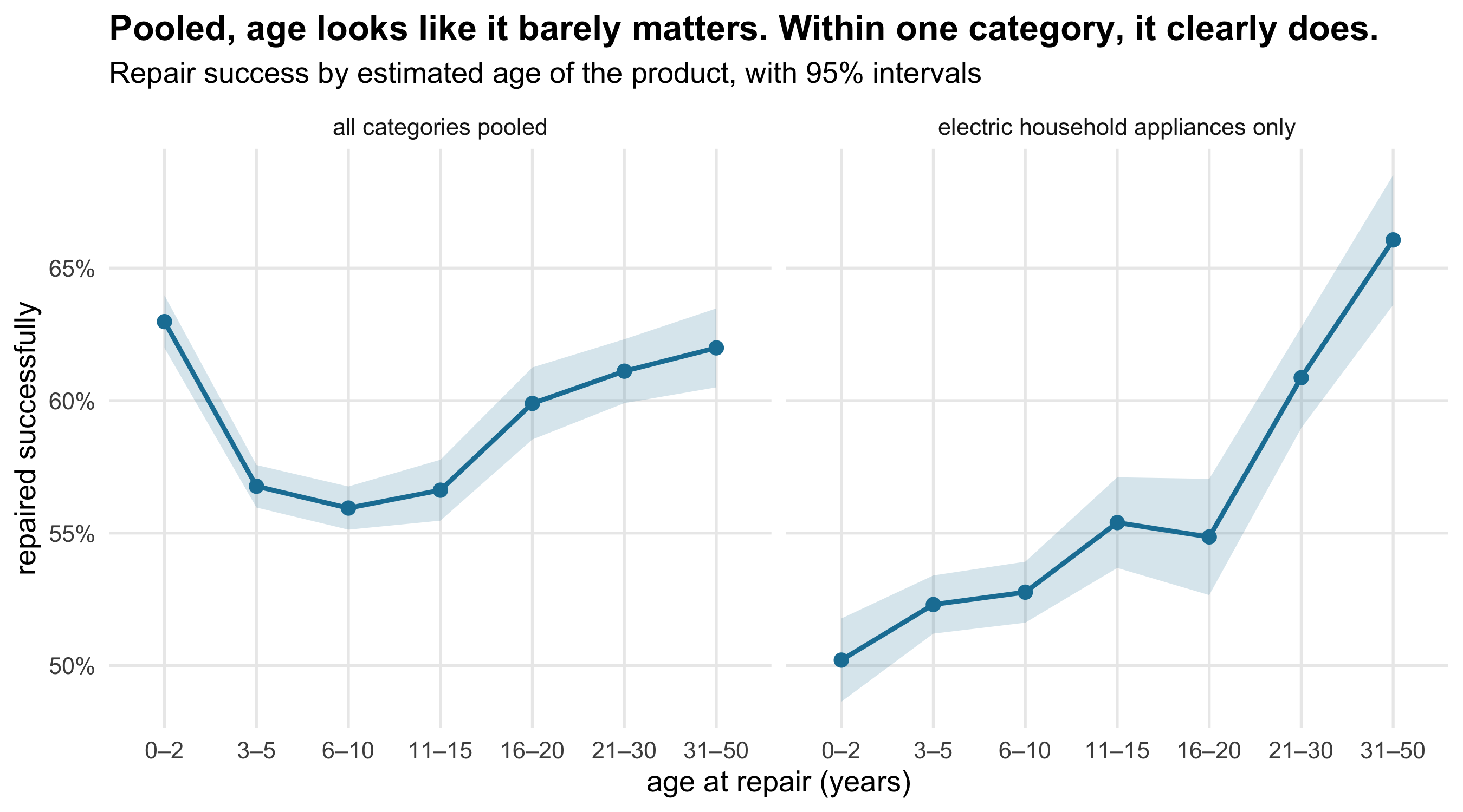
Pooled across everything, the age curve is a shallow U — worst in the middle, slightly
better at both ends — which mostly reflects *what* is old. Thirty-year-old objects arriving
at a Repair Café skew towards furniture and hand tools; three-year-old ones skew towards
consumer electronics. The pooled line is measuring the changing category mix as much as
age.
Hold the category fixed and the picture sharpens. Among electric household appliances
alone, success climbs steadily with age: `r af("0–2")` for appliances under three years old,
`r af("21–30")` for those over twenty. On this evidence, an old washing machine really is a
better bet than a new one.
::: {.callout-note}
## Why I would not call that planned obsolescence
The within-category comparison removes the category-mix confound. It does not remove three
others, and they all push the same way.
**Survivorship.** A twenty-five-year-old appliance that is still in someone's kitchen has
already survived twenty-five years without being thrown away. It is, by construction, a
good one. The new appliances in this data are a full cross-section of new appliances; the
old ones are the survivors of their cohort.
**Different faults.** Old machines tend to arrive with worn belts, perished seals and dead
switches. New ones arrive with control-board faults. That is a real difference in
repairability, but it is a difference in *what went wrong*, not necessarily in how well the
thing was built.
**Informative missingness.** Estimated production year is recorded for only
`r sprintf("%.0f%%", 100*mean(!is.na(repairs$estimated_year_of_production)))` of attempts,
and the items that have it are fixed `r mf(TRUE)` of the time against `r mf(FALSE)` for
those that don't. Whatever decides whether a volunteer writes down the age is correlated
with the outcome, so every age figure on this page is computed on a non-random third of the
data.
The honest reading is that older appliances in this dataset are more repairable, and that
at least three mechanisms other than declining build quality would produce exactly that.
:::
## Answer three: the reason written on the form
When a repair fails, volunteers record why. This is the part with policy attached.
```{r failures}
#| fig-height: 5
#| fig-cap: "Recorded reasons a repair could not be completed, grouped by whether the obstacle is a property of the product's design and supply chain."
reasons <- read_csv("data/repairs_text.csv", show_col_types = FALSE) |>
  filter(!is.na(failure_reasons)) |>
  count(failure_reasons, sort = TRUE) |>
  mutate(
    kind = if_else(
      str_detect(failure_reasons, "Spare parts|open the product|information"),
      "designed in", "intrinsic to the object or the session"),
    failure_reasons = fct_reorder(failure_reasons, n)
  )

share_design <- sum(reasons$n[reasons$kind == "designed in"]) / sum(reasons$n)

ggplot(reasons, aes(n, failure_reasons, fill = kind)) +
  geom_col(width = 0.72) +
  scale_fill_manual(values = c("designed in" = "#c75146",
                               "intrinsic to the object or the session" = "#1a7fa3"),
                    name = NULL) +
  scale_x_continuous(labels = scales::comma,
                     expand = expansion(mult = c(0, 0.08))) +
  labs(
    title = sprintf("%.0f%% of failed repairs were stopped by parts or access",
                    100 * share_design),
    subtitle = paste0("Reasons recorded for ", format(sum(reasons$n), big.mark = ","),
                      " incomplete repairs"),
    x = "times recorded", y = NULL
  ) +
  theme(legend.position = "top",
        panel.grid.major.y = element_blank(),
        plot.title = element_text(face = "bold"))
```
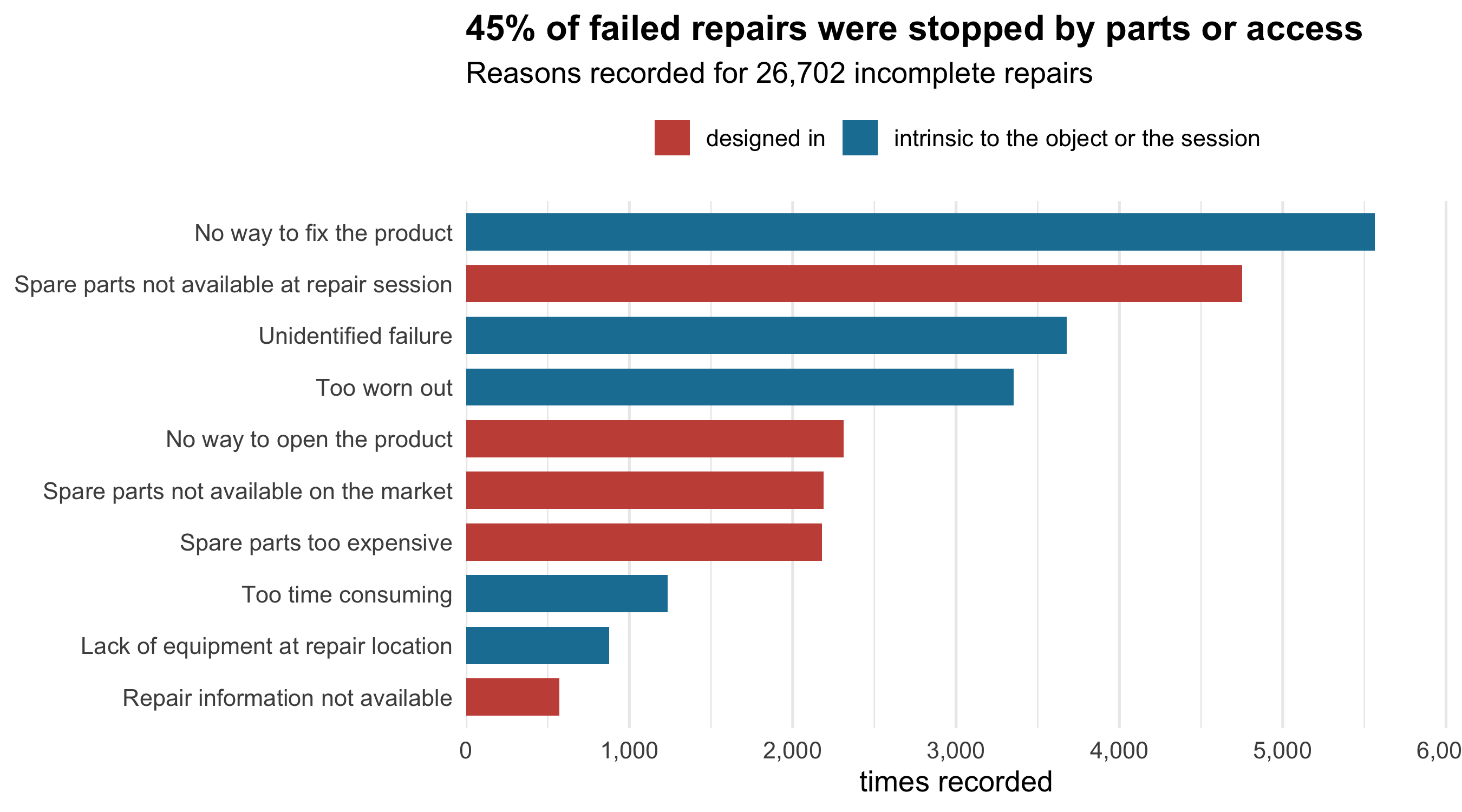
Three of the reasons are properties of the object as it was designed and sold: **spare parts
weren't available** (at the session, on the market, or at a sane price), **the product could
not be opened**, and **repair information did not exist**. Together they account for
`r sprintf("%.0f%%", 100*share_design)` of recorded failures.
These are precisely the three things right-to-repair legislation targets: parts
availability, non-destructive disassembly, and published service documentation. This dataset
is not an argument for that legislation — the people filling in these forms are volunteers
with a view. But it is a measurement of how often the obstacle was the *design* rather than
the damage, and the answer is: most of the time.
## A footnote on the volunteers' own judgement
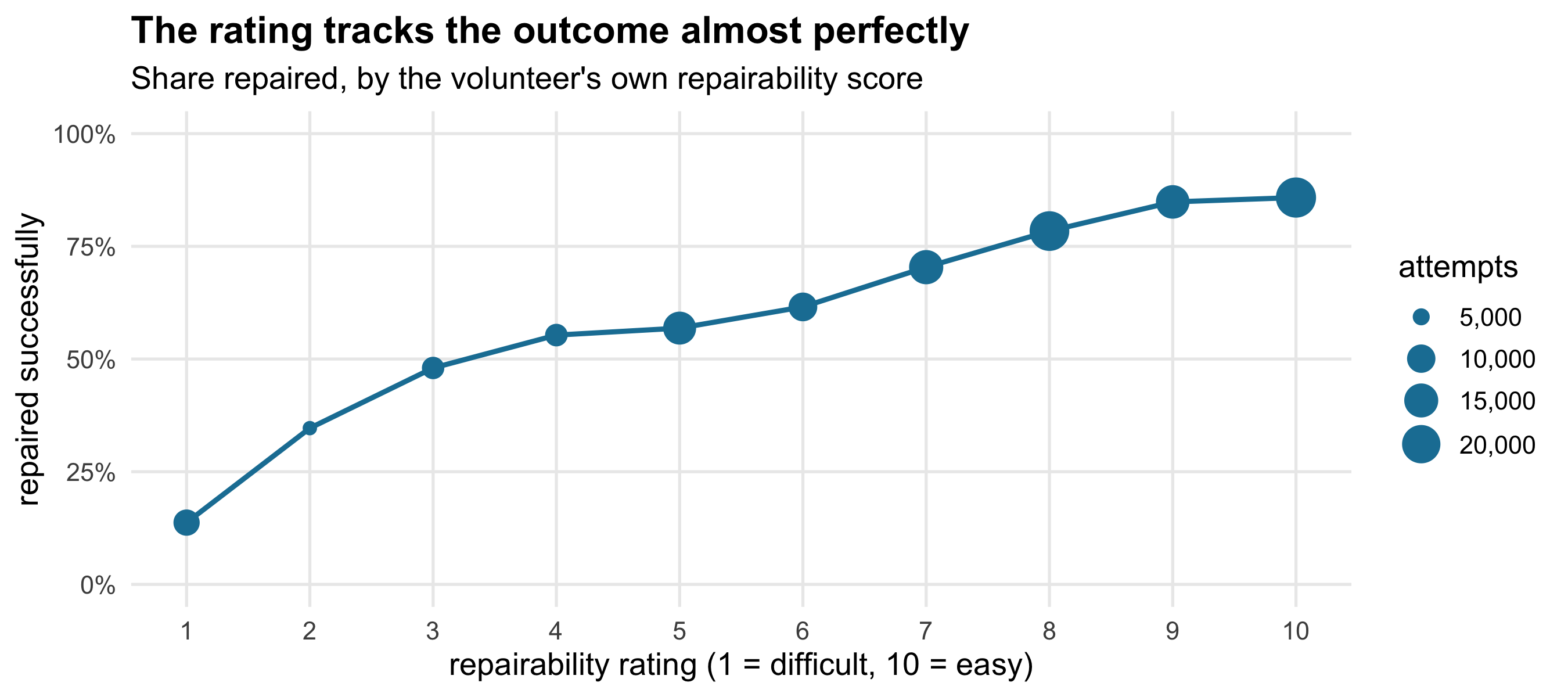
Each attempt carries a "repairability" score from 1 to 10, recorded by the person doing the
work.
```{r calibration}
#| fig-height: 4
#| fig-cap: "Observed repair success against the volunteer's 1–10 repairability rating."
calib <- repairs |>
  filter(!is.na(repairability), between(repairability, 1, 10)) |>
  summarise(n = n(), fixed = mean(fixed), .by = repairability)

ggplot(calib, aes(repairability, fixed)) +
  geom_line(colour = "#1a7fa3", linewidth = 1) +
  geom_point(aes(size = n), colour = "#1a7fa3") +
  scale_x_continuous(breaks = 1:10) +
  scale_y_continuous(labels = scales::percent, limits = c(0, 1)) +
  scale_size_continuous(range = c(2, 7), labels = scales::comma, name = "attempts") +
  labs(
    title = "The rating tracks the outcome almost perfectly",
    subtitle = "Share repaired, by the volunteer's own repairability score",
    x = "repairability rating (1 = difficult, 10 = easy)", y = "repaired successfully"
  ) +
  theme(plot.title = element_text(face = "bold"),
        panel.grid.minor = element_blank())
```
From `r sprintf("%.0f%%", 100*calib$fixed[calib$repairability==1])` at a rating of 1 to
`r sprintf("%.0f%%", 100*calib$fixed[calib$repairability==10])` at 10, monotonically. It is
tempting to call this well-calibrated expert judgement.
I don't think we can. Nothing in the data says when the rating was written down, and the
natural moment to record how hard something was to repair is *after* trying. If so, this
figure is not a forecast being validated but a description agreeing with itself — which is
a much less impressive thing, and indistinguishable from the impressive version with the
data as published.
::: {.callout-note}
## What this can and cannot say
**These are not representative products.** Everything here is an object someone thought was
worth carrying to a café to save. Products that are cheap enough to replace, or obviously
beyond hope, never enter the data. Repair rates on this page are conditional on someone
already believing a repair was plausible.
**Nor a representative world.** Just over half the records come from the Netherlands, with
the UK and France next; the network's culture, volunteer skill and parts access are not
global constants. Country is not controlled for anywhere on this page.
**"Fixed" is self-reported, at the table.** It records that the object worked when it left
the room, not that it was still working a month later. Partial repairs
(`r sprintf("%.0f%%", 100*mean(repairs$outcome == "partly fixed"))` of attempts) are
counted as not fixed throughout, which is a choice: counting them as successes would raise
every rate on this page by roughly ten points without changing any of the comparisons.
**Failure reasons exist only for failures, and only sometimes.** Of
`r format(sum(!repairs$fixed), big.mark = ",")` unsuccessful attempts, about
`r sprintf("%.0f%%", 100*sum(reasons$n)/sum(!repairs$fixed))` carry a recorded reason. If volunteers
are likelier to write down a tidy institutional reason ("spare parts not available") than a
vague one, the design-related share is overstated.
:::