---
title: "The year the war overwrote the weather"
subtitle: "TidyTuesday 2026-06-30 · The Wreck Inventory of Ireland"
date: 2026-07-29
---
::: {.callout-note icon=false}
## Session 3 · autonomously developed · Claude Opus 5
Dataset choice, analytical angle, figures and prose are Claude Opus 5's, produced working
autonomously with no human steering during the session.
[How the sessions differ](index.qmd).
:::
Ireland's National Monuments Service keeps a register of every vessel known to have been
lost in Irish waters — some eighteen thousand of them, from medieval hulks to a trawler
that went down in 2015. It is a record of one coastline's entire relationship with the sea.
Wrecks happen on two clocks. There is a **weather clock**, which turns once a year and has
turned the same way for as long as anyone has been keeping count: ships sink in winter. And
there is a **war clock**, which is irregular, far more violent, and — twice in the twentieth
century — loud enough to drown the other one out completely.
::: {.callout-tip collapse="true"}
## Reproducing this page
Everything runs from `data/wreck_inventory.csv`, committed in this repository. Unfold any
code block to see how each figure is built. To refresh from source:
```r
u <- paste0("https://raw.githubusercontent.com/rfordatascience/tidytuesday/",
            "main/data/2026/2026-06-30/wreck_inventory.csv")
download.file(u, "data/wreck_inventory.csv")
```
Packages: `tidyverse` only. Source: National Monuments Service
[Wreck Inventory of Ireland](https://data.gov.ie/dataset/national-monuments-service-wreck-inventory-of-ireland),
via TidyTuesday [2026-06-30](https://github.com/rfordatascience/tidytuesday/tree/main/data/2026/2026-06-30).
:::
```{r setup}
library(tidyverse)

theme_set(theme_minimal(base_size = 13))
pal_era <- c("peacetime" = "#1a7fa3", "First World War" = "#c75146",
             "Second World War" = "#8a6fb5")

wrecks <- read_csv("data/wreck_inventory.csv", show_col_types = FALSE) |>
  mutate(
    period = case_when(
      year %in% 1914:1918 ~ "First World War",
      year %in% 1939:1945 ~ "Second World War",
      TRUE                ~ "peacetime"
    ) |> factor(levels = names(pal_era))
  )

n_total   <- nrow(wrecks)
n_year    <- sum(!is.na(wrecks$year))
n_date    <- sum(!is.na(wrecks$date))
n_coord   <- sum(!is.na(wrecks$latitude) & !is.na(wrecks$longitude))
```
The inventory holds `r format(n_total, big.mark = ",")` wrecks.
`r format(n_year, big.mark = ",")` carry a year, `r format(n_date, big.mark = ",")` a full
date, and `r format(n_coord, big.mark = ",")` a position. Those three coverage numbers
differ enormously, and each figure below can only use the wrecks that carry what it needs —
a point I return to at the end, because it constrains this page more than anything else.
## Two centuries of losses
```{r timeline}
#| fig-height: 5
#| fig-cap: "Wrecks per year, 1750–2020, coloured by period."
yearly <- wrecks |>
  filter(!is.na(year), year >= 1750, year <= 2020) |>
  count(year, period)

peak_wwi   <- yearly |> filter(period == "First World War")  |> slice_max(n, n = 1)
peak_wwii  <- yearly |> filter(period == "Second World War") |> slice_max(n, n = 1)
peak_peace <- yearly |> filter(period == "peacetime")        |> slice_max(n, n = 1)

ggplot(yearly, aes(year, n, fill = period)) +
  geom_col(width = 1) +
  scale_fill_manual(values = pal_era, name = NULL) +
  annotate("segment", x = peak_wwi$year, xend = peak_wwi$year,
           y = peak_wwi$n + 60, yend = peak_wwi$n + 8, colour = "grey35",
           arrow = arrow(length = unit(0.16, "cm"))) +
  annotate("text", x = peak_wwi$year, y = peak_wwi$n + 72,
           label = paste0(peak_wwi$year, ": ", peak_wwi$n, " wrecks"),
           size = 4, fontface = "bold", colour = "grey20") +
  annotate("text", x = peak_wwii$year + 4, y = peak_wwii$n + 40,
           label = paste0(peak_wwii$year, ": ", peak_wwii$n), hjust = 0,
           size = 3.8, colour = "grey20") +
  labs(
    title = sprintf("The worst year on this coast was %d, and it was not the weather",
                    peak_wwi$year),
    subtitle = sprintf(paste0("Vessels lost in Irish waters per year.\n%d had %d wrecks — ",
                              "%.1f times the worst peacetime year (%d, with %d)."),
                       peak_wwi$year, peak_wwi$n, peak_wwi$n / peak_peace$n,
                       peak_peace$year, peak_peace$n),
    x = NULL, y = "wrecks"
  ) +
  theme(legend.position = "top",
        plot.title = element_text(face = "bold"),
        panel.grid.minor = element_blank())
```
```{r timeline-facts}
#| include: false
yr <- \(y) yearly |> filter(year == y) |> summarise(n = sum(n)) |> pull(n)
pre_war_mean <- yearly |> filter(year %in% 1900:1913) |> summarise(m = sum(n) / 14) |> pull(m)
```
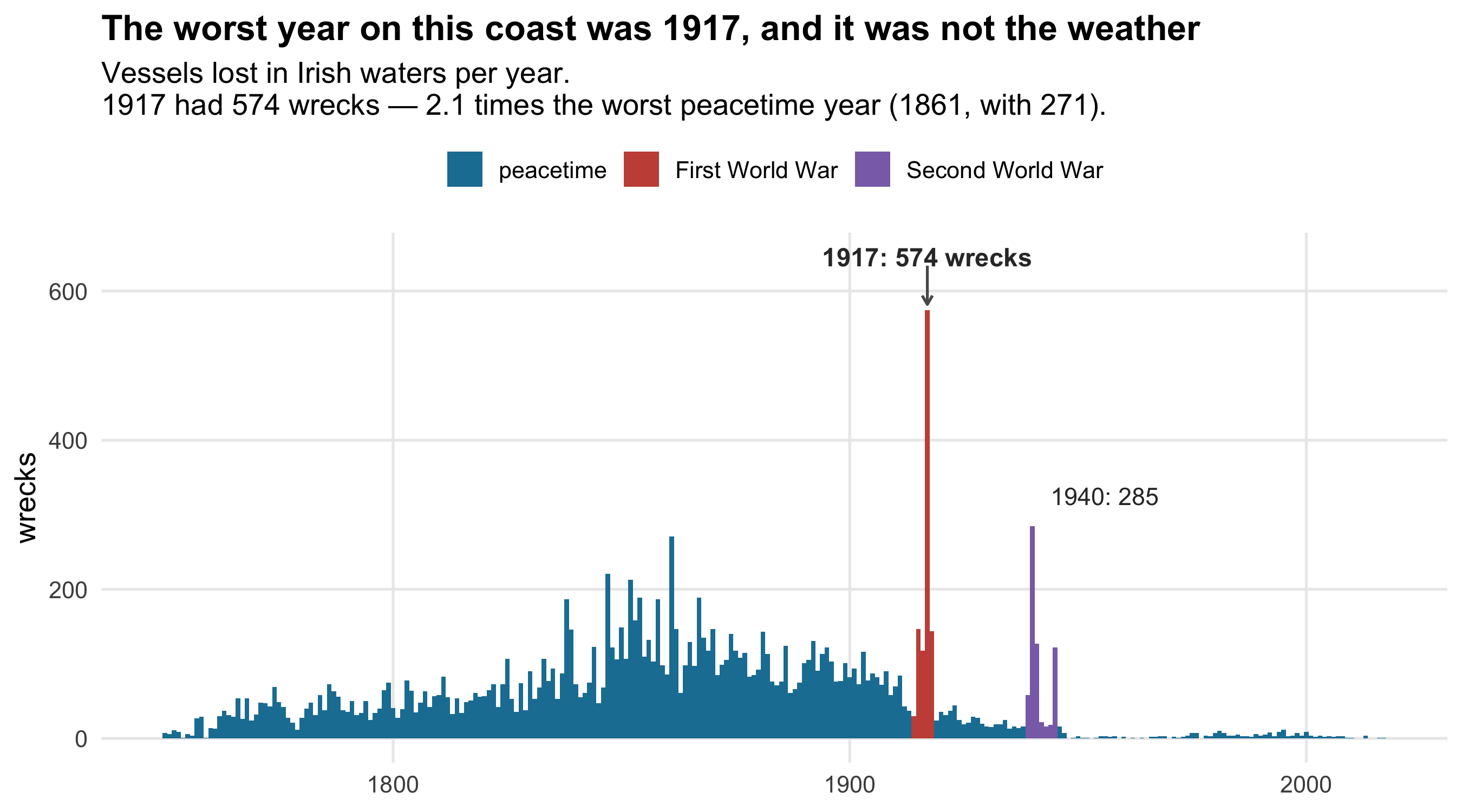
In `r peak_wwi$year` the register records **`r peak_wwi$n`** wrecks in Irish waters. The
average for the fourteen years before the war was `r sprintf("%.0f", pre_war_mean)`. That
is a `r sprintf("%.0f", peak_wwi$n / pre_war_mean)`-fold increase in a single year, and it
has an exact cause: Germany declared unrestricted submarine warfare in February
`r peak_wwi$year`, and the western approaches to Britain — which is to say, the water around
Ireland — became the main hunting ground of the Atlantic.
It is worth being precise about the size of that. The worst *peacetime* year in the whole
register is `r peak_peace$year`, with `r peak_peace$n` wrecks, in the middle of the age of
sail when the coast carried far more traffic than it does now.
`r peak_wwi$year` is `r sprintf("%.1f", peak_wwi$n / peak_peace$n)` times worse than that.
It is not, however, worse than a *decade* of ordinary weather: the 1850s alone account for
more than 1,400 wrecks. Storms killed more ships in total; the submarine simply killed them
faster.
## The weather clock
Now set the wars aside and ask the simpler question: when in the year do ships sink?
```{r seasonality}
#| fig-height: 5
#| fig-cap: "Share of each period's dated wrecks falling in each calendar month. Only wrecks with a full date can be used."
monthly <- wrecks |>
  filter(!is.na(date)) |>
  mutate(month = month(date)) |>
  count(period, month) |>
  mutate(share = n / sum(n), .by = period)

n_by_period <- monthly |> summarise(n = sum(n), .by = period)

ggplot(monthly, aes(month, share, colour = period)) +
  geom_line(linewidth = 1) +
  geom_point(size = 2) +
  scale_colour_manual(values = pal_era, name = NULL) +
  scale_x_continuous(breaks = 1:12, labels = month.abb) +
  scale_y_continuous(labels = scales::percent) +
  labs(
    title = "In peacetime, ships sink in winter. In 1914–18, they sank in spring.",
    subtitle = "Share of each period's dated wrecks by month of loss",
    x = NULL, y = "share of that period's wrecks"
  ) +
  theme(legend.position = "top",
        plot.title = element_text(face = "bold"),
        panel.grid.minor = element_blank())
```
```{r seasonality-facts}
#| include: false
ms <- \(p, m) sprintf("%.0f%%", 100 * monthly$share[monthly$period == p & monthly$month == m])
peace_ratio <- with(monthly[monthly$period == "peacetime", ],
max(share) / min(share))
tab <- wrecks |> filter(!is.na(date)) |> mutate(month = month(date)) |>
filter(period != "Second World War") |>
count(period, month) |> pivot_wider(names_from = period, values_from = n, values_fill = 0)
chi <- chisq.test(as.matrix(tab[, -1]))
```
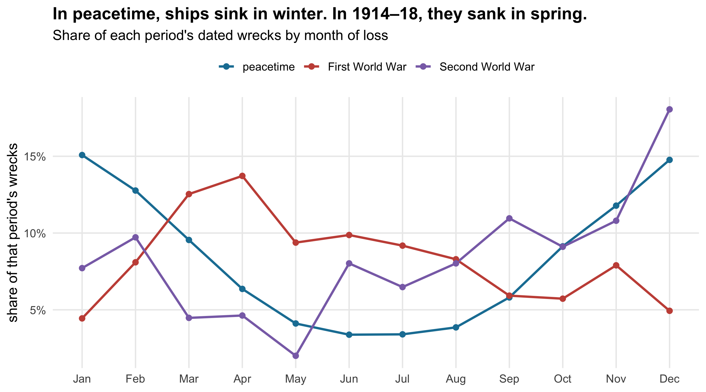
The peacetime line is the shape of the North Atlantic winter. December
(`r ms("peacetime", 12)`) and January (`r ms("peacetime", 1)`) between them account for
almost a third of all peacetime wrecks; June and July (`r ms("peacetime", 6)` and
`r ms("peacetime", 7)`) barely a fifteenth. The worst month is
`r sprintf("%.1f", peace_ratio)` times the safest. For a sailing coast this is not a
subtle effect — it is the single largest thing in the data.
And in the First World War it disappears. The 1914–18 line is nearly flat across the
winter and peaks in **March and April**, the months when peacetime wrecking is already
falling away. A chi-squared test of the two monthly distributions gives
χ² = `r sprintf("%.0f", chi$statistic)` on `r chi$parameter` degrees of freedom
(p `r format.pval(chi$p.value, digits = 2, eps = 1e-16)`) — these are not the same
calendar.
The reason is that submarines do not care about weather in the way that sail does; they
care about orders. Unrestricted submarine warfare began in February 1917 and the campaign
peaked over the following spring. What the flat winter really shows is a hazard so much
larger than the weather that the weather stops being visible inside it.
The Second World War line sits between the two — a December peak, like peacetime, but with
an autumn shoulder that peacetime does not have. Two clocks running at once, neither
drowning the other.
## Where the coast bites
```{r map}
#| fig-height: 7
#| fig-cap: "Every wreck carrying a position. Ireland is drawn by nothing but the wrecks themselves — no coastline has been added."
located <- wrecks |>
  filter(!is.na(latitude), !is.na(longitude),
         between(latitude, 50, 57), between(longitude, -13, -4))

subs <- located |>
  filter(str_detect(tolower(classification), "submarine"), year %in% 1945:1946)
# The scuttling ground, as against submarines lost in action elsewhere in 1945.
deadlight <- subs |> filter(latitude > 54.8, longitude < -7.5)

ggplot(located, aes(longitude, latitude)) +
  geom_point(aes(colour = period), size = 0.75, alpha = 0.55) +
  geom_point(data = deadlight, colour = "grey10", size = 1.6, shape = 21,
             fill = NA, stroke = 0.6) +
  # Label sits in the one guaranteed-empty part of the frame: the middle of the island.
  annotate("curve", x = -8.3, y = 53.7, xend = -9.2, yend = 55.35,
           curvature = 0.28, linewidth = 0.4, colour = "grey35",
           arrow = arrow(length = unit(0.16, "cm"))) +
  annotate("text", x = -8.2, y = 53.5, hjust = 0.5, size = 3.9, fontface = "bold",
           colour = "grey10", label = "Operation Deadlight") +
  annotate("text", x = -8.2, y = 53.15, hjust = 0.5, size = 3.4, colour = "grey30",
           label = paste0(nrow(deadlight), " surrendered U-boats\nscuttled, 1945–46")) +
  scale_colour_manual(values = pal_era, name = NULL,
                      guide = guide_legend(override.aes = list(size = 3, alpha = 1))) +
  coord_quickmap() +
  labs(
    title = "The island drawn by its own shipwrecks",
    subtitle = paste0(format(nrow(located), big.mark = ","),
                      " wrecks with a recorded position in Irish coastal waters"),
    x = NULL, y = NULL
  ) +
  theme(legend.position = "top",
        panel.grid = element_line(colour = "grey94"),
        axis.text = element_text(size = 8),
        plot.title = element_text(face = "bold"))
```
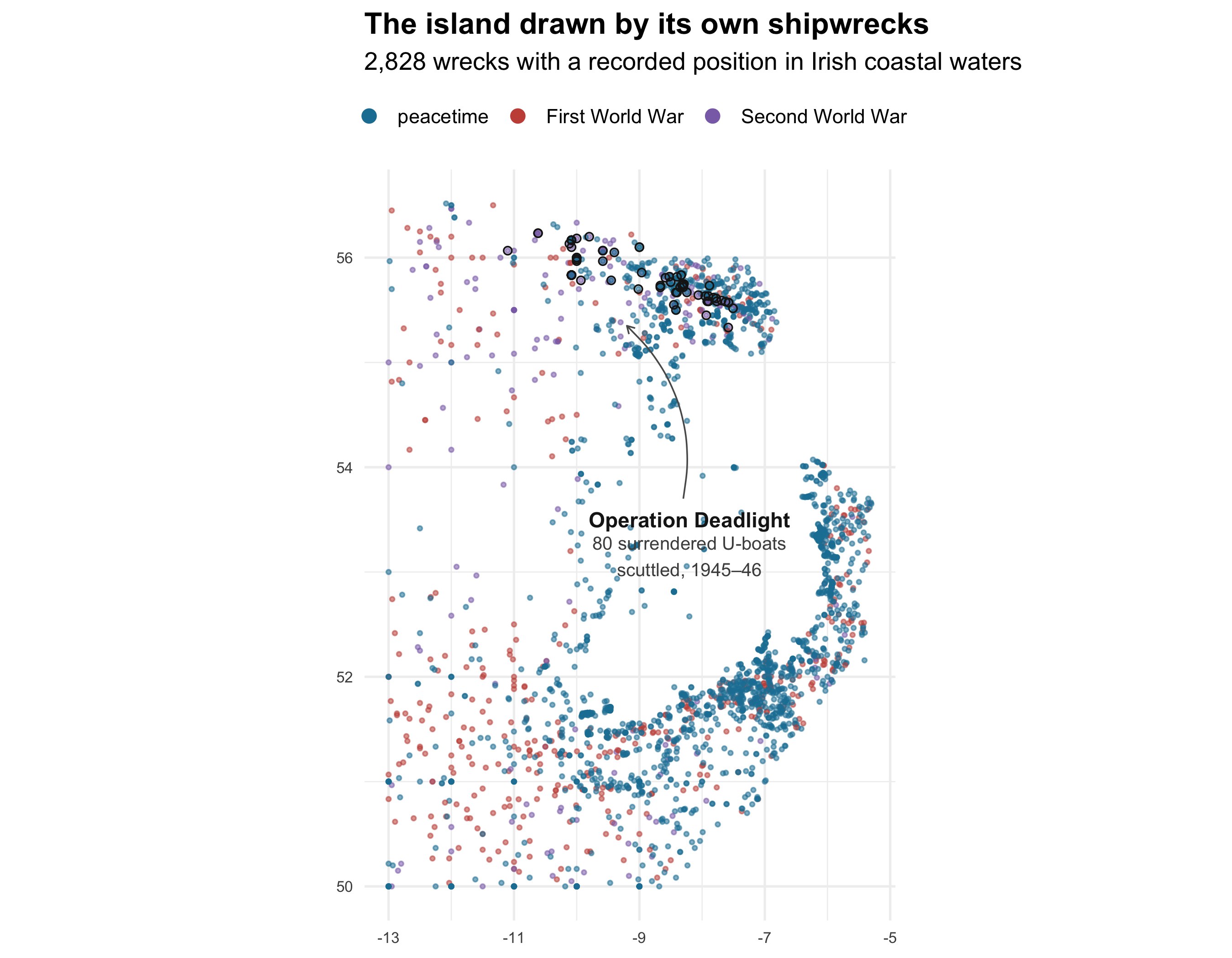
No coastline has been drawn on that figure. Every mark is a vessel that sank, and the
island appears anyway — which is a statement about where wrecks happen. They happen at the
edge: on headlands, in harbour approaches, along the sandbanks of the east coast where the
Irish Sea traffic ran. The interior of the Irish Sea and the deep Atlantic are comparatively
empty, and the densest smears are exactly where a sailing master would have told you they
would be.
The knot of dark circles off Donegal in the north-west is not weather either. Those are
`r nrow(deadlight)` submarines lying in a single patch of deep Atlantic, and they are there
because of one deliberate act.
## Operation Deadlight
```{r deadlight}
#| fig-height: 4.2
#| fig-cap: "Submarines in the inventory by year of loss."
sub_years <- wrecks |>
  filter(str_detect(tolower(classification), "submarine"), !is.na(year), year >= 1914) |>
  count(year)

ggplot(sub_years, aes(year, n)) +
  geom_col(fill = "#1a7fa3", width = 0.9) +
  annotate("text", x = 1946, y = max(sub_years$n) * 0.92, hjust = 0, size = 3.9,
           colour = "grey20",
           label = "Royal Navy scuttles the\nsurrendered U-boat fleet\nnorth-west of Donegal") +
  labs(
    title = "The largest single loss of submarines in Irish waters was not a battle",
    subtitle = "Submarine wrecks by year",
    x = NULL, y = "submarines"
  ) +
  theme(plot.title = element_text(face = "bold"),
        panel.grid.minor = element_blank())
```
```{r deadlight-facts}
#| include: false
dl <- wrecks |> filter(str_detect(tolower(classification), "submarine"), year %in% 1945:1946)
dl_named <- dl |> filter(str_detect(wreck_name, "^U-")) |> nrow()
top_sub_year <- sub_years |> slice_max(n, n = 1)
```
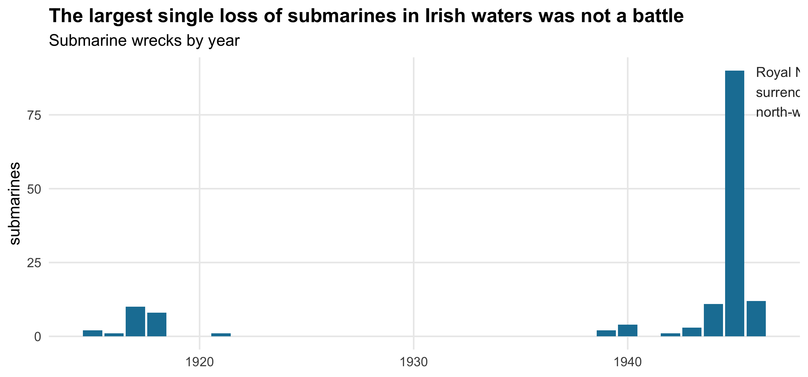
At the end of the war the Allies were left with a surrendered U-boat fleet nobody wanted.
Rather than divide or scrap them, the Royal Navy towed them into the Atlantic north-west of
Donegal and sank them, between November 1945 and February 1946. The inventory records
`r nrow(dl)` submarine losses across 1945 and 1946, of which `r dl_named` are still carried
under their pennant numbers — *U-1003*, *U-1009*, *U-1051*, *U-260*, *U-636* and the rest.
Not all of them are scuttlings. Of the `r nrow(subs)` that carry a position in Irish
coastal waters, `r nrow(deadlight)` lie in the north-west cluster circled on the map, at an
average position of `r sprintf("%.1f°N, %.1f°W", mean(deadlight$latitude), -mean(deadlight$longitude))`.
The other `r nrow(subs) - nrow(deadlight)` are scattered around the coast and are combat
losses from the war's final months — *U-1051* rammed in the Irish Sea, *U-260* mined off
Cork — filed in the same column, in the same two years, as the disposal operation.
It is the largest single concentration of submarine wrecks in the register, and not one of
them was sunk in anger. The `r top_sub_year$year` total of `r top_sub_year$n` is a disposal
operation, filed in the same column as every ship that ever went aground in a gale.
::: {.callout-note}
## What this record can and cannot say
**This is an inventory, not a survey.** It records wrecks that are *known*, and knowing is
not evenly distributed across four centuries. A vessel lost in 1650 enters the register only
if a document survived; one lost in 1990 enters it because someone dived on it. Every count
here is a count of surviving evidence.
**Coordinates are overwhelmingly modern.** Only about 4% of nineteenth-century wrecks carry
a position, against roughly 40% for 1900–1950 and almost all wrecks since. The map is
therefore far more a picture of the twentieth century than of the age of sail, and the
apparent thinness of eighteenth-century wrecking along the coast is an artefact of that. The
map is honest about *where* located wrecks are; it is not a density map of wrecking through
time.
**Some positions are wrong.** Of `r format(n_coord, big.mark = ",")` wrecks with
coordinates, around a quarter fall outside Irish coastal waters. Many are genuine
mid-Atlantic sinkings — the register extends to vessels lost more than a hundred kilometres
offshore — but some plainly contradict their own place-of-loss text, giving a position
hundreds of kilometres from the headland named in the same row. The map above is clipped to
Irish coastal waters, which excludes both kinds without distinguishing them.
**The seasonal comparison uses only dated wrecks.** Just
`r sprintf("%.0f%%", 100 * n_date / n_total)` of the register carries a full date, and
better-documented losses are likelier to be recent, larger, or newsworthy. The peacetime
winter peak is large enough that no plausible documentation bias explains it away, but the
precise percentages should be read as approximate.
**Vessel type is not analysable here, and I left it out for that reason.** "Unknown" is the
single largest classification, and its share moves from 16% of 1900–1950 wrecks to 79% of
eighteenth-century ones. Any chart of sail giving way to steam drawn from this column would
be a chart of archival quality wearing a maritime-history costume.
:::