---
title: "Birth is scheduled: calendar effects in 15 years of US births"
subtitle: "TidyTuesday 2018-10-02 · Daily US births, 2000–2014"
date: 2026-06-09
---
::: {.callout-tip icon=false}
## Session 1 · co-developed
This page came out of a live, turn-by-turn conversation between Jon Minton and Claude
(Fable 5) — questions, plots and interpretation built together in real time. The
[Session 2 pages](index.qmd) were instead produced by Claude working autonomously.
:::
Every daily birth count in the United States from 2000 to 2014 — 5,479 days. Births
feel like the most natural, least controllable of events, yet at the population scale
the calendar's fingerprints are everywhere. This dataset is really about *obstetric
scheduling*: the modern machinery of inductions and planned caesareans, which bends
the timing of birth toward the working week and away from holidays.
```{r setup}
library(tidyverse)

dow_names <- c("Mon", "Tue", "Wed", "Thu", "Fri", "Sat", "Sun")

births <- read_csv("data/us_births.csv", show_col_types = FALSE) |>
  mutate(
    date = as.Date(sprintf("%d-%02d-%02d", year, month, date_of_month)),
    dow = factor(dow_names[day_of_week], levels = dow_names),
    weekend = day_of_week >= 6
  )

theme_set(theme_minimal(base_size = 13))
```
## The working-week birth
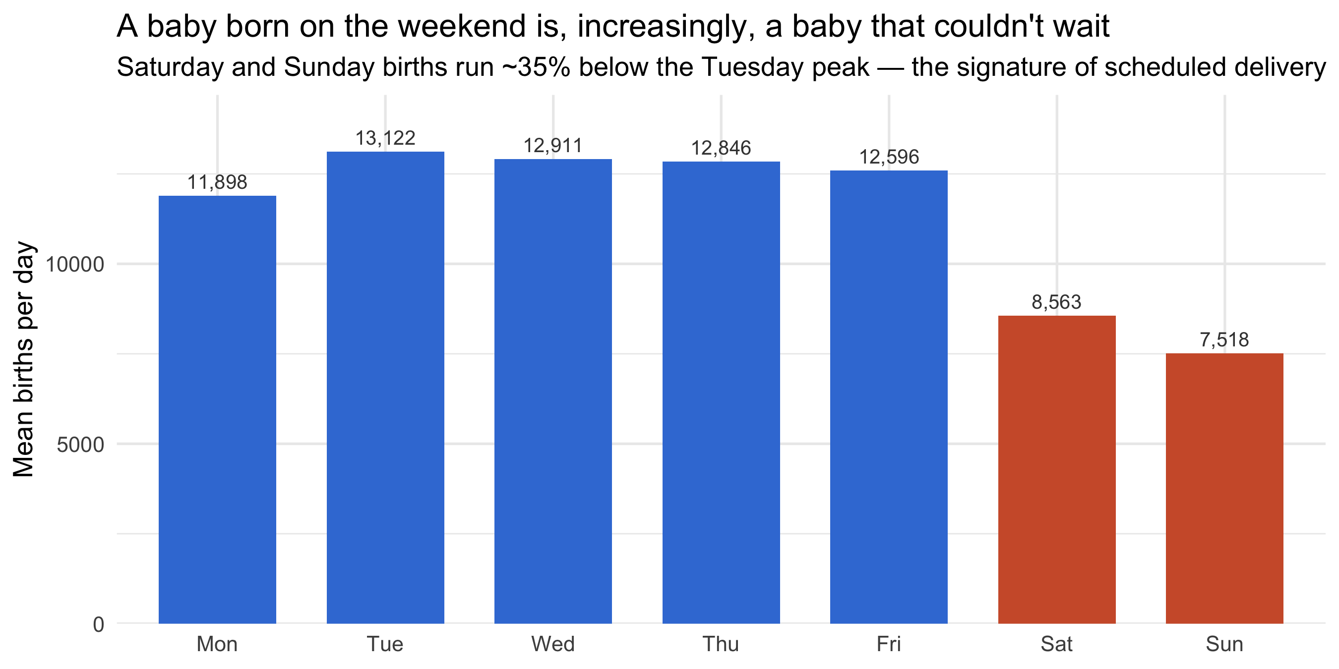
The single largest signal in the data isn't seasonal — it's weekly. Average daily
births collapse at the weekend, because elective inductions and caesareans are
booked Monday to Friday.
```{r weekday}
#| fig-height: 4.5
#| fig-cap: "Average daily births by day of week, 2000–2014. Weekend births run roughly a third below weekday births."
births |>
  summarise(mean_births = mean(births), .by = dow) |>
  ggplot(aes(dow, mean_births, fill = dow %in% c("Sat", "Sun"))) +
  geom_col(width = 0.7) +
  geom_text(aes(label = scales::comma(round(mean_births))),
            vjust = -0.5, size = 3.4, colour = "grey25") +
  scale_fill_manual(values = c("#3b7dd8", "#cf5c36"), guide = "none") +
  scale_y_continuous(expand = expansion(c(0, 0.12))) +
  labs(
    title = "A baby born on the weekend is, increasingly, a baby that couldn't wait",
    subtitle = "Saturday and Sunday births run ~35% below the Tuesday peak — the signature of scheduled delivery",
    x = NULL, y = "Mean births per day"
  )
```
## A year of births, day by day
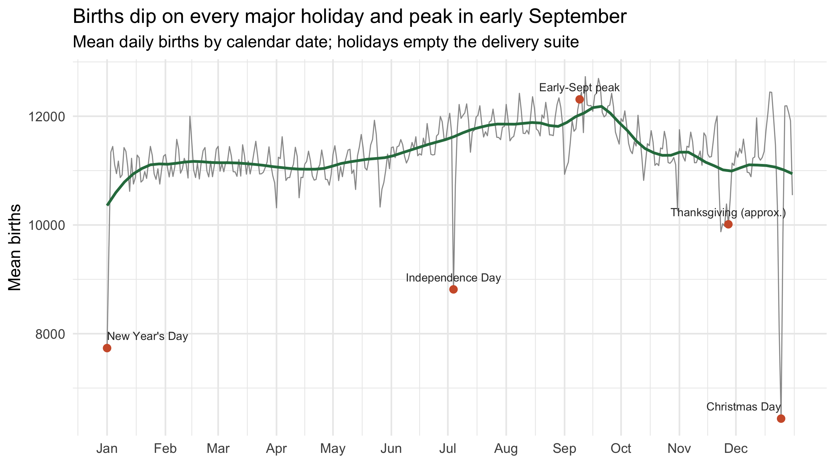
Averaging each calendar date across the 15 years reveals the holidays as sharp
troughs — and a few telling spikes.
```{r calendar-ribbon}
#| fig-height: 5
#| fig-cap: "Mean births by day of the year (averaged 2000–2014). Notable dates annotated."
doy <- births |>
  mutate(md = format(date, "%m-%d")) |>
  filter(md != "02-29") |>
  summarise(mean_births = mean(births), .by = md) |>
  mutate(doy = row_number())

marks <- tibble::tribble(
  ~md,      ~label,
  "01-01",  "New Year's Day",
  "07-04",  "Independence Day",
  "12-25",  "Christmas Day",
  "11-27",  "Thanksgiving (approx.)",
  "09-09",  "Early-Sept peak"
) |>
  left_join(doy, by = "md")

ggplot(doy, aes(doy, mean_births)) +
  geom_line(colour = "grey60", linewidth = 0.4) +
  geom_smooth(se = FALSE, colour = "#2c7a4d", span = 0.18, linewidth = 1) +
  geom_point(data = marks, colour = "#cf5c36", size = 2.3) +
  geom_text(
    data = marks, aes(label = label), size = 3.1, colour = "grey20",
    vjust = -1, hjust = c(0, 0.5, 1, 0.5, 0.5)
  ) +
  scale_x_continuous(
    breaks = cumsum(c(1, 31, 28, 31, 30, 31, 30, 31, 31, 30, 31, 30)),
    labels = month.abb
  ) +
  labs(
    title = "Births dip on every major holiday and peak in early September",
    subtitle = "Mean daily births by calendar date; holidays empty the delivery suite",
    x = NULL, y = "Mean births"
  )
```
The early-September peak is real and recurring (a December–January conception
window, much debated). But the troughs are the cleaner story: Christmas, New
Year, Independence Day and Thanksgiving all show steep dips — the same scheduling
hand as the weekend effect, pulling planned deliveries away from public holidays.
## The unluckiest day to be born
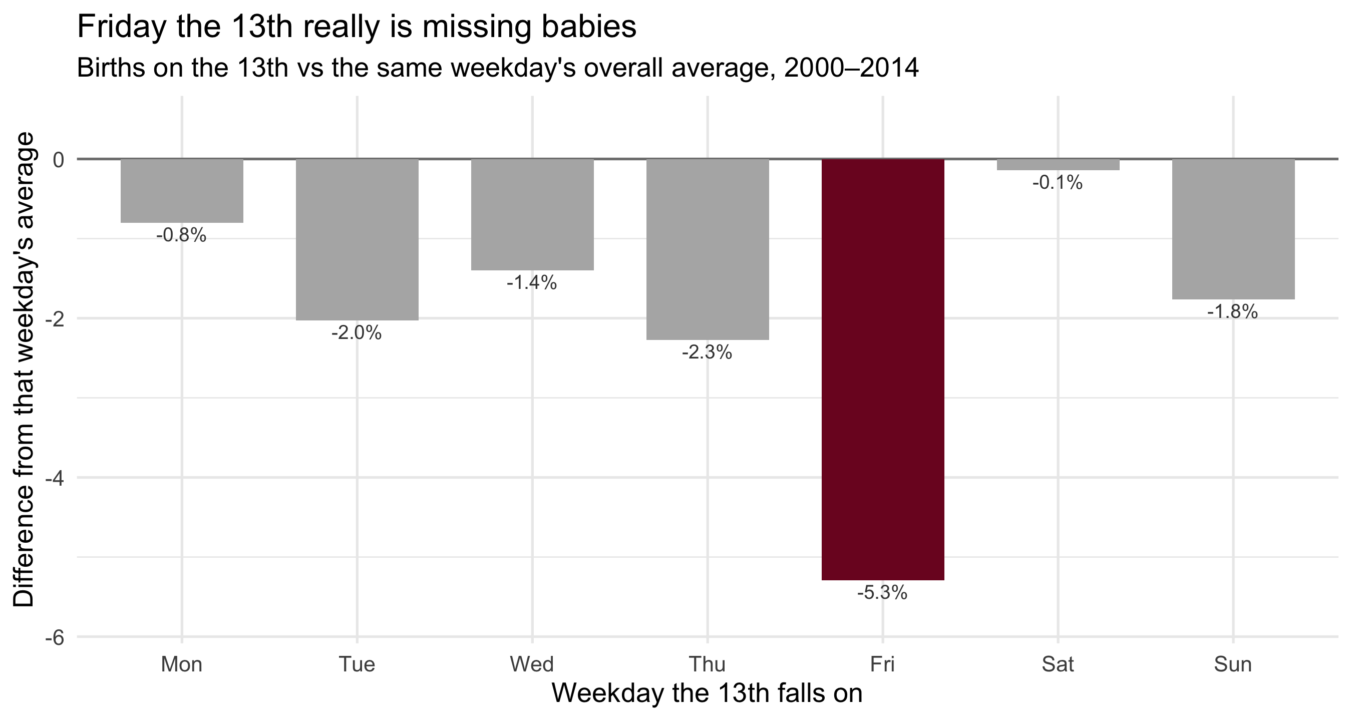
If birth timing is partly chosen, do people avoid *unlucky* dates? The 13th of the
month lets us test it — and Friday the 13th most of all.
```{r friday-13}
#| fig-height: 4.8
#| fig-cap: "Births on the 13th relative to the same weekday's average. Friday the 13th stands out."
f13 <- births |>
  mutate(is13 = date_of_month == 13) |>
  summarise(m = mean(births), .by = c(dow, is13)) |>
  pivot_wider(names_from = is13, values_from = m,
              names_prefix = "x") |>
  mutate(pct = 100 * (xTRUE / xFALSE - 1))

ggplot(f13, aes(dow, pct, fill = dow == "Fri")) +
  geom_hline(yintercept = 0, colour = "grey50") +
  geom_col(width = 0.7) +
  geom_text(aes(label = sprintf("%+.1f%%", pct),
                vjust = ifelse(pct < 0, 1.3, -0.5)),
            size = 3.3, colour = "grey25") +
  scale_fill_manual(values = c("grey70", "#7d1128"), guide = "none") +
  scale_y_continuous(expand = expansion(0.15)) +
  labs(
    title = "Friday the 13th really is missing babies",
    subtitle = "Births on the 13th vs the same weekday's overall average, 2000–2014",
    x = "Weekday the 13th falls on", y = "Difference from that weekday's average"
  )
```
Every 13th sees slightly fewer births than its weekday norm, but **Friday the
13th is the outlier at −5.3%** — more than double the next-largest dip. With the
weekday already held constant, this isn't the weekend effect in disguise: it's a
measurable reluctance to schedule a delivery on a day folklore marks as unlucky.
A small, superstitious distortion in the timing of something we like to think of
as beyond our control.
::: {.callout-note}
## A note on the test
Comparing the 13th to *the same weekday's* average is the key control — a naive
"13th vs all days" comparison would confound the date with whatever weekday it
happened to fall on. Holding weekday fixed isolates the date superstition from
the much larger weekly scheduling cycle.
:::