Jon Minton’s Blog - Part Six: The Robo-Chauffeur

Aim

In the previous post in this series, I presented a function for calculating the log likelihood of a standard linear regression with a Normal error term. I then built a very simple dataset, ten data points linking \(x\) to \(y\), and showed how the log likelihood varied as a combination of different candidate values for the model’s intercept and slope terms (\(\beta_0\) and \(\beta_1\) respectively).

The aim of this this post is to show how the best parameter combinations tend to be estimated from a model’s log likelihood in practice, using an optimisation algorithm that iteratively tries out new parameter values, and keeps trying and trying until some kind of condition is met. This is what the last figure in the first post is trying to illustrate.

Optimisation algorithms: getting there faster

In the previous post, we ‘cheated’ a bit when using the log likelihood function, fixing the value for one of the parameters \(\sigma^2\) to the value we used when we generated the data, so we could instead look at how the log likelihood surface varied as different combinations of \(\beta_0\) and \(\beta_1\) were plugged into the formula. \(\beta_0\) and \(\beta_1\) values ranging from -5 to 5, and at steps of 0.1, were considered: 101 values of \(\beta_0\), 101 values of \(\beta_1\), and so over 10,000¹ unique \(\{\beta_0, \beta_1\}\) combinations were stepped through. This approach is known as grid search, and seldom used in practice (except for illustration purposes) because the number of calculations involved can very easily get out of hand. For example, if we were to use it to explore as many distinct values of \(\sigma^2\) as we considered for \(\beta_0\) and \(\beta_1\), the total number of \(\{\beta_0, \beta_1, \sigma^2 \}\) combinations we would crawl through would be over 100,000 ² rather than over 10,000.

One feature we noticed with the likelihood surface over \(\beta_0\) and \(\beta_1\) in the previous post is that it appears to look like a hill, with a clearly defined highest point (the region of maximum likelihood) and descent in all directions from this highest point. Where likelihood surfaces have this feature of being single-peaked in this way (known as ‘unimodal’), then a class of algorithms known as ‘hill climbing algorithms’ can be applied to find the top of such peaks in a way that tends to be both quicker (fewer steps) and more precise than the grid search approach used for illustration in the previous post.

Code recap

Let’s copy over the code we used in the previous post for:

1. Calculating log likelihood

Code

llNormal <- function(pars, y, X){
    beta <- pars[1:ncol(X)]
    sigma2 <- exp(pars[ncol(X)+1])
    -1/2 * (sum(log(sigma2) + (y - (X%*%beta))^2 / sigma2))
}

And

1. Generating our tame toy dataset of 10 data points

Code

# set a seed so runs are identical
set.seed(7)
# create a main predictor variable vector: -3 to 5 in increments of 1
x <- (-3):5
# Record the number of observations in x
N <- length(x)
# Create a response variable with variability
y <- 2.5 + 1.4 * x  + rnorm(N, mean = 0, sd = 0.5)

# bind x into a two column matrix whose first column is a vector of 1s (for the intercept)

X <- cbind(rep(1, N), x)
# Clean up names
colnames(X) <- NULL

To recap, the toy dataset looks as follows:

Code

library(tidyverse)
tibble(x=x, y=y) |>
    ggplot(aes(x, y)) + 
    geom_point()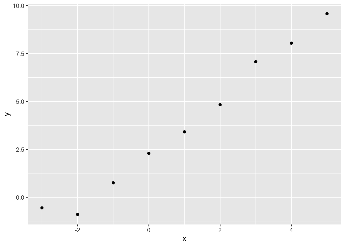

`optim`: our Robo-Chauffeur

Note how the llNormal function takes a single argument, pars, which packages up all the specific candidate parameter values we want to try out. In our previous post, we also had a ‘feeder function’, feed_to_ll, which takes the various \(\beta\) candidate values from the grid and packages them into pars. In our previous post, we had to specify the candidate values to try to feed to llNormal packages inside pars.

But we don’t have to do this. We can instead use an algorithm to take candidate parameters, try them out, then make new candidate parameters and try them out, for us. Much as a taxi driver needs to know where to meet a passenger, but doesn’t want the passenger to tell them exactly which route to take, we just need to specify a starting set of values for the parameters to optimise. R’s standard way of doing this is with the optim function. Here’s it in action:

Code

optim_results <-  optim(
    # par contains our initial guesses for the three parameters to estimate
    par = c(0, 0, 0), 

    # by default, most optim algorithms prefer to search for a minima (lowest point) rather than maxima 
    # (highest point). So, I'm making a function to call which simply inverts the log likelihood by multiplying 
    # what it returns by -1
    fn = function(par, y, X) {-llNormal(par, y, X)}, 

    # in addition to the par vector, our function also needs the observed output (y)
    # and the observed predictors (X). These have to be specified as additional arguments.
    y = y, X = X
    )

optim_results

$par
[1]  2.460571  1.375421 -1.336209

$value
[1] -1.51397

$counts
function gradient 
     216       NA 

$convergence
[1] 0

$message
NULL

The optim function returns a fairly complex output structure, with the following components:

par: the values for the parameters (in our case \(\{\beta_0, \beta_1, \eta \}\)) which the optimisation algorithm ended up with.
value: the value returned by the function fn when the optim routine was stopped.
counts: the number of times the function fn was repeatedly called by optim before optim decided it had had enough
convergence: whether the algorithm used by optim completed successfully (i.e. reached what it considers a good set of parameter estimates in par), or not.

In this case, convergence is 0, which (perhaps counterintuitively) indicates a successful completion. counts indicates that optim called the log likelihood function 216 times before stopping, and par indicates values of \(\{\beta_0 = 2.46, \beta_1 = 1.38, \eta = -1.34\}\) were arrived at. As \(\sigma^2 = e^\eta\), this means \(\theta = \{\beta_0 = 2.46, \beta_1 = 1.38, \sigma^2 = 0.26 \}\). As a reminder, the ‘true’ values are \(\{\beta_0 = 2.50, \beta_1 = 1.40, \sigma^2 = 0.25\}\).

So, the optim algorithm has arrived at pretty much the correct answers for all three parameters, in 216 calls to the log likelihood function, whereas for the grid search approach in the last post we made over 10,000 calls to the log likelihood function for just two of the three parameters.

Let’s see if we can get more information on exactly what kind of path optim took to get to this set of parameter estimates. We should be able to do this by specifying a value in the trace component in the control argument slot…

Comparisons

For comparison let’s see what lm and glm produce.

First lm:

Code

toy_df <- tibble(
    x = x, 
    y = y
)


mod_lm <- lm(y ~ x, data = toy_df)
summary(mod_lm)


Call:
lm(formula = y ~ x, data = toy_df)

Residuals:
    Min      1Q  Median      3Q     Max 
-0.6082 -0.3852 -0.1668  0.2385  1.1092 

Coefficients:
            Estimate Std. Error t value Pr(>|t|)    
(Intercept)  2.46067    0.20778   11.84 6.95e-06 ***
x            1.37542    0.07504   18.33 3.56e-07 ***
---
Signif. codes:  0 '***' 0.001 '**' 0.01 '*' 0.05 '.' 0.1 ' ' 1

Residual standard error: 0.5813 on 7 degrees of freedom
Multiple R-squared:  0.9796,    Adjusted R-squared:  0.9767 
F-statistic:   336 on 1 and 7 DF,  p-value: 3.564e-07

\(\{\beta_0 = 2.46, \beta_1 = 1.38\}\), i.e. the same to 2 decimal places.

And now with glm:

Code

mod_glm <- glm(y ~ x, data = toy_df, family = gaussian(link = "identity"))

summary(mod_glm)


Call:
glm(formula = y ~ x, family = gaussian(link = "identity"), data = toy_df)

Coefficients:
            Estimate Std. Error t value Pr(>|t|)    
(Intercept)  2.46067    0.20778   11.84 6.95e-06 ***
x            1.37542    0.07504   18.33 3.56e-07 ***
---
Signif. codes:  0 '***' 0.001 '**' 0.01 '*' 0.05 '.' 0.1 ' ' 1

(Dispersion parameter for gaussian family taken to be 0.3378601)

    Null deviance: 115.873  on 8  degrees of freedom
Residual deviance:   2.365  on 7  degrees of freedom
AIC: 19.513

Number of Fisher Scoring iterations: 2

Once again, \(\{\beta_0 = 2.46, \beta_1 = 1.38\}\)

Discussion

In the above, we’ve successfully used optim, our Robo-Chauffeur, to arrive very quickly at some good estimates for our parameters of interest, \(\beta_0\) and \(\beta_1\), which are in effect identical to those produced by the lm and glm functions.

This isn’t a coincidence. What we’ve done the hard way is what the glm function (in particular) largely does ‘under the hood’.

Coming up

In the next part of this series, we’ll see how other outputs available from optim can be used to estimate uncertainty in the parameters of interest, how this information can be used to produce the kinds of estimates of standard errors around coefficients which are summarised in glm and lm summary() functions, and which many (ab)users of statistical models obsess about when star-gazing, and how information about uncertainty in parameter estimates allows for more honest model-based predictions.

Footnotes

\(101^2 = 10201\)↩︎
\(101^3 = 1030301\)↩︎

Aim

Optimisation algorithms: getting there faster

Code recap

optim: our Robo-Chauffeur

Comparisons

Discussion

Coming up

Footnotes

`optim`: our Robo-Chauffeur