Interactive Sliders with Crosstalk and Plotly

Introduction

Below is an example of creating a plotly chart with an interactive slider using crosstalk.

By default, the plot shows the proportion of datazones in a local authority that are in the 15% most deprived datazones in Scotland. (Using the 2020 SIMD).

The slider allows different thresholds than the 15% default to be selected.

Data Downloading and Preparation

To see the code itself, just click on the word ‘code’ to open up the block’.

Code

library(tidyverse)
library(plotly)
library(crosstalk)
library(here)

Code

if(!file.exists(here("simd_data.xlsx"))){
  download.file(
    url = "https://www.gov.scot/binaries/content/documents/govscot/publications/statistics/2020/01/scottish-index-of-multiple-deprivation-2020-data-zone-look-up-file/documents/scottish-index-of-multiple-deprivation-data-zone-look-up/scottish-index-of-multiple-deprivation-data-zone-look-up/govscot%3Adocument/SIMD%2B2020v2%2B-%2Bdatazone%2Blookup.xlsx",
    destfile = here("simd_data.xlsx"),
    mode = "wb"
  )
}

dta <- openxlsx::readWorkbook(here("simd_data.xlsx"), sheet = "SIMD 2020v2 DZ lookup data")

The code for the figure itself is below. It’s quite a convoluted process. There’s almost certaintly neater ways of doing this. The main thing to keep in mind is all the figures exist; just only one is visible at a time.

Code

# So let's construct a new aval containing the different x-y tuples given the threshold selected

calc_prop_deprived <- function(q, dta){
    dta %>% 
      group_by(HBname) %>% 
      summarise(prop_deprived = mean(pct_rank < q)) %>% 
      ungroup()
}

df_rank <- 
  dta %>% 
    select(HBname, SIMD2020v2_Rank) %>% 
    mutate(pct_rank = SIMD2020v2_Rank / max(SIMD2020v2_Rank))


shared_df <- tibble(
  dep_quants = seq(0.05, 0.95, by = 0.05)
) %>% 
  mutate(derived_props = map(dep_quants, calc_prop_deprived, dta = df_rank)) %>% 
  unnest(derived_props) %>% 
  mutate(undep_quants = 1 - dep_quants) 


# Now to put it in the structure, and set active for `dep_quants = 0.15`


unique_dep_quants <- unique(shared_df$dep_quants)
n_steps <- length(unique_dep_quants)

dep_vals <- list()
for (step in 1:n_steps){
  tmp <- 
    shared_df %>% 
      filter(dep_quants == unique_dep_quants[step]) %>% 
      select(HBname, prop_deprived) %>% 
      mutate(HBname = reorder(HBname, prop_deprived))
  
  dep_vals[[step]] <- list(
    visible = FALSE,
    name = paste0('Quantile: ', unique_dep_quants[step]),
    x=tmp$prop_deprived,
    y=tmp$HBname
    
  ) 
}

# 15% is the third list object 

dep_vals[3][[1]]$visible = TRUE

# Now visualise 

# create steps and plot all traces
dep_steps <- list()
fig <- plot_ly() 
for (i in c(3, 1, 2, 4:n_steps)) { # Start with 3 as this is 15% and this should determine the default HB order 
 fig <- add_bars(fig,x=dep_vals[i][[1]]$x,  y=dep_vals[i][[1]]$y, visible = dep_vals[i][[1]]$visible, 
                 name = dep_vals[i][[1]]$name, orientation = 'h', hoverinfo = 'x+y', color = I("gray"),
                 showlegend = FALSE) %>% 
   layout(
      title = list(
        text = glue::glue("Proportion of datazones in Health Boards at least this deprived")
      ),
      xaxis = list(
        title = "Proportion this deprived in Health Board",
        range = list(0, 1)
      ),
      yaxis = list(
        title = "Health Board"
      )
   )

  step <- list(args = list('visible', rep(FALSE, length(dep_vals))),
               method = 'restyle')
  step$args[[2]][i] = TRUE  
  step$label = unique_dep_quants[i]
  dep_steps[[i]] = step 
}  
#names(dep_steps) <- unique_dep_quants

fig <- fig %>%
  layout(sliders = list(list(active = 2,
                             currentvalue = list(prefix = "Deprivation: "),
                             steps = dep_steps)))

fig

As you can see, there’s still some work to do regarding formatting. But it works!

Static

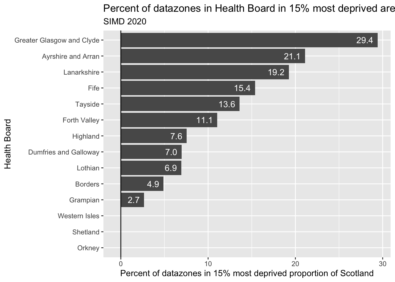
For comparison, here’s the same data used to produce a static plot

Code

# Now to put it in the structure, and set active for `dep_quants = 0.15`

df_15pc <- shared_df |> 
  filter(between(dep_quants, 0.149, 0.151)) |> 
  select(-dep_quants, -undep_quants)

df_15pc |>
  mutate(pct_deprived = 100 * prop_deprived) |> 
  ggplot(aes(y= pct_deprived, x = fct_reorder(HBname, pct_deprived))) + 
  geom_bar(stat = "identity") +
  geom_text(
    aes(
      label = ifelse(df_15pc$prop_deprived > 0, sprintf("%.1f", pct_deprived), "")
    ), 
    color = "white",
    hjust = 1, 
    nudge_y = -0.5
  ) + 
  coord_flip() + 
  labs(
    x = "Health Board",
    y = "Percent of datazones in 15% most deprived proportion of Scotland",
    title = "Percent of datazones in Health Board in 15% most deprived areas of Scotland",
    subtitle = "SIMD 2020"
  ) + 
  geom_hline(yintercept = 0)