Scientific Illustrations: Annotating the unit circle

Here’s an example of a scientific illustration I’ve just produced to illustrate some scenarios I’m modelling for my work on economic inactivity determinants.

I have two continuous variables (derived from the GHQ-12), mental health and physical health. Both are standardised so they have the same scale.

But I’m interested in the effects of improving/changing ‘health’ in general, which is obviously composed of both mental health and physical health, but not measured directly.

As the two variables are standardised, however, I can model an improvement in health in general as a change in both mental health and physical health concurrently.

However, I want to compare like-with-like: scenarios in which the total ‘amount’ of intervention effect is kept constant, but the relative contribution of the two health components is varied.

This is where a little trigonometry comes in. ¹ All interventions on the grey unit circle in Figure 1 represent possible scenarios in which the total amount of health change is constant, but where the relative contribution of mental and physical health is varied.

The aim of the scientific illustration is to make this intuition a bit clearer to understand!

Code

library(tidyverse)
library(geomtextpath)

pos_y <- function(x) {sqrt(1 - x^2)}
x = seq(0, 1, by = 0.001)
dta <- tibble(
  x = x
) |> 
  mutate(
    y = pos_y(x)
  )

dta |> 
  ggplot(aes(x = x, y = y)) + 
    geom_line(color = "grey") + 
    coord_equal() + 
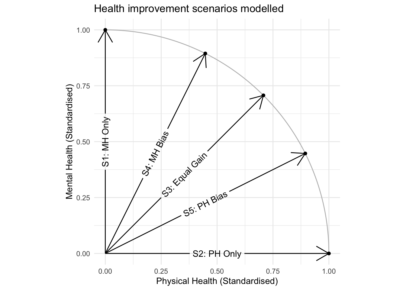
    labs(x = "Physical Health (Standardised)",
         y = "Mental Health (Standardised)",
         title = "Health improvement scenarios modelled") + 
  theme_minimal() + 
  annotate("point", x = 1, y = 0) + 
  annotate("point", x = 0, y = 1) + 
  annotate("point", x = 1/ sqrt(2), y = 1/ sqrt(2)) + 
  annotate("point", x =  2 / sqrt(5), y = 1 / sqrt(5)) + 
  annotate("point", x = 1 / sqrt(5), y = 2 / sqrt(5)) + 
  geom_textcurve(
    data = data.frame(x = 0, y = 0, xend = 0, yend = 1), 
                      mapping = aes(x, y, xend = xend,  yend = yend), 
                      label = "S1: MH Only", 
    curvature = 0, hjust = 0.5, arrow = arrow(),
    vjust = 0.5
  ) + 
  geom_textcurve(
    data = data.frame(x = 0, y = 0, xend = 1, yend = 0), 
                      mapping = aes(x, y, xend = xend,  yend = yend), 
                      label = "S2: PH Only", 
    curvature = 0, hjust = 0.5, arrow = arrow(),
    vjust = 0.5
  ) + 
  geom_textcurve(
    data = data.frame(x = 0, y = 0, xend = 1/sqrt(2), yend = 1/sqrt(2)), 
                      mapping = aes(x, y, xend = xend,  yend = yend), 
                      label = "S3: Equal Gain", 
    curvature = 0, hjust = 0.5, arrow = arrow(),
    vjust = 0.5
  ) + 
  geom_textcurve(
    data = data.frame(x = 0, y = 0, yend = 2/sqrt(5), xend = 1/sqrt(5)), 
                      mapping = aes(x, y, xend = xend,  yend = yend), 
                      label = "S4: MH Bias", 
    curvature = 0, hjust = 0.5, arrow = arrow(),
    vjust = 0.5
  )  +
  geom_textcurve(
    data = data.frame(x = 0, y = 0, yend = 1/sqrt(5), xend = 2/sqrt(5)), 
                      mapping = aes(x, y, xend = xend,  yend = yend), 
                      label = "S5: PH Bias", 
    curvature = 0, hjust = 0.5, arrow = arrow(),
    vjust = 0.5
  )  

Figure 1: Modelling various intervention scenarios

Footnotes

1. People who claim you’ll never need trigonometry once you leave school are wrong. It’s valuable about once a decade!