A shorter and even tardier Tidy Tuesday this week, given we gave ourselves only half an hour rather than the usual hour to look over the most recent dataset.
The dataset was about Christmas films.
Our first question: is Die Hard a Christmas film?
Not according to the methods used to produce the dataset . If a film doesn’t have Christmas or equivalent in its title, it’s not coming in!
<- tidytuesdayR:: tt_load ('2023-12-12' )
---- Compiling #TidyTuesday Information for 2023-12-12 ----
--- There are 2 files available ---


── Downloading files ───────────────────────────────────────────────────────────

  1 of 2: "holiday_movies.csv"
  2 of 2: "holiday_movie_genres.csv"
<- tt[[1 ]]<- tt[[2 ]]
%>% count (year, sort = TRUE )
# A tibble: 91 × 2
    year     n
   <dbl> <int>
 1  2021   183
 2  2022   173
 3  2020   172
 4  2019   143
 5  2018   129
 6  2023   107
 7  2017   102
 8  2015    76
 9  2016    75
10  2012    68
# ℹ 81 more rows
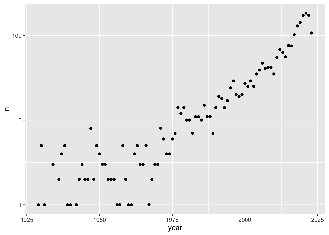
how many films by year -plot with log on y axis
%>% count (year) %>% ggplot (aes (x = year, y = n))+ geom_point ()+ #stat_smooth()+ scale_y_log10 ()
how many films by year -plot with log on y axis
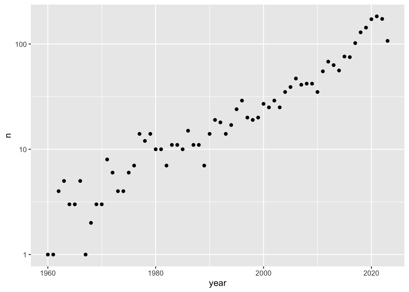
filter by 1960 onwards
%>% filter (year >= 1960 ) %>% count (year) %>% ggplot (aes (x = year, y = n))+ geom_point ()+ #stat_smooth()+ scale_y_log10 ()
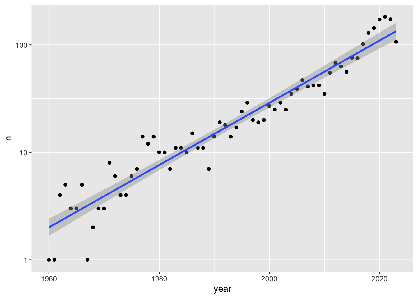
how many films by year -plot with log on y axis
filter by 1960 onwards
%>% filter (year >= 1960 ) %>% count (year) %>% ggplot (aes (x = year, y = n))+ geom_point ()+ stat_smooth (method = "lm" )+ scale_y_log10 ()
`geom_smooth()` using formula = 'y ~ x'
questions
how are they published? [cinema / streaming?]
is it on imdb?
full inclusion of 2023?
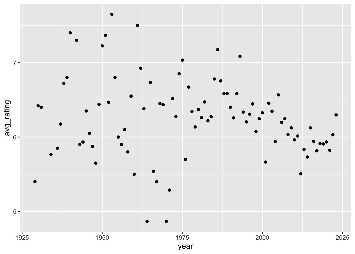
are more recent films rubbish?
%>% group_by (year) %>% summarise (avg_rating = mean (average_rating)) %>% ggplot (aes (x = year, y = avg_rating))+ geom_point ()
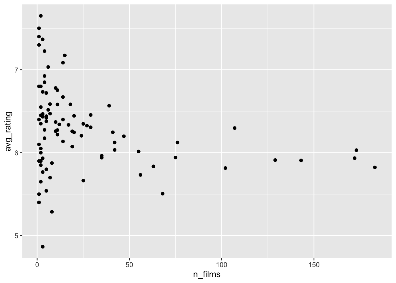
number of films vs avg rating
fewer films may drive extreme values
number of films vs avg rating
%>% group_by (year) %>% summarise (avg_rating = mean (average_rating), n_films = n () ) %>% ggplot (aes (x = n_films, y = avg_rating))+ geom_point ()