library(tidyverse)
library(ggbeeswarm) # for the beeswarm plotBackground
This week’s TidyTuesday used data from the UK ONS which was explored in the 2023 article ’Why do children and young people in smaller towns do better academically than those in larger towns?’.
Aims
Our first aim was to try to replicate the headline finding from the article above: that children in smaller towns have better average educational outcomes than in larger towns. We also sought to replicate and improve on the ‘beeswarm’ plot used in the original article, and to look at other factors which may explain differences in educational qualifications.
Package loading
Data
# ee <- tidytuesdayR::tt_load('2024-01-23') |>
#   purrr::pluck(1)

# Direct link to get past API rate limit issue using tt_load()
ee <- readr::read_csv('https://raw.githubusercontent.com/rfordatascience/tidytuesday/master/data/2024/2024-01-23/english_education.csv')
purrr::pluck(1) was used because the data contained only a single dataset, but by default the tt_load function returns a list. So, the pluck(1) function takes the first element of the list, which in this case is in effect turning the data into a dataframe.
Counting towns in data
ee |>
  count(size_flag, sort=T) |>
knitr::kable(caption = "Counts of small/med/city class")| size_flag | n |
|---|---|
| Small Towns | 662 |
| Medium Towns | 331 |
| Large Towns | 89 |
| City | 18 |
| Inner London BUA | 1 |
| Not BUA | 1 |
| Other Small BUAs | 1 |
| Outer london BUA | 1 |
There are 662 small towns, 331 medium towns, and 89 large towns
Removing oddball locations and Londons and factoring
ee |>
  mutate(town_size = factor(size_flag, levels = c("Small Towns", "Medium Towns", "Large Towns"), ordered=T)) |>
  filter(!is.na(town_size)) -> ee_fact
Summary by group
ee_fact |>
  group_by(town_size) |>
  summarise(count = n(),
            `mean ed score` = mean(education_score),
            `sd ed score` = sd(education_score),
            se = `sd ed score`/count^0.5,
            `total population` = sum(population_2011)) |>
  mutate(across(where(is.numeric), round, 3)) |>
  knitr::kable()
Warning: There was 1 warning in `mutate()`.
ℹ In argument: `across(where(is.numeric), round, 3)`.
Caused by warning:
! The `...` argument of `across()` is deprecated as of dplyr 1.1.0.
Supply arguments directly to `.fns` through an anonymous function instead.
# Previously
across(a:b, mean, na.rm = TRUE)
# Now
across(a:b, \(x) mean(x, na.rm = TRUE))| town_size | count | mean ed score | sd ed score | se | total population |
|---|---|---|---|---|---|
| Small Towns | 662 | 0.297 | 3.887 | 0.151 | 6880216 |
| Medium Towns | 331 | -0.253 | 3.324 | 0.183 | 12213733 |
| Large Towns | 89 | -0.811 | 2.298 | 0.244 | 10466343 |
ANOVA for small/med/large towns
We built a series of linear regression models, and used ANOVA to compare between them. A low p-value from ANOVA, when comparing two or more models that are ‘nested’, can be taken as a signal that the more complex/unrestricted of the models should be used.
mod_base <- lm(education_score ~ town_size, data = ee_fact)
summary(mod_base)
Call:
lm(formula = education_score ~ town_size, data = ee_fact)

Residuals:
     Min       1Q   Median       3Q      Max
-10.3246  -2.5270  -0.1996   2.3052  11.5749

Coefficients:
             Estimate Std. Error t value Pr(>|t|)
(Intercept) -0.255991   0.151293  -1.692  0.09093 .
town_size.L -0.783553   0.288560  -2.715  0.00673 **
town_size.Q -0.003547   0.232530  -0.015  0.98783
---
Signif. codes:  0 '***' 0.001 '**' 0.01 '*' 0.05 '.' 0.1 ' ' 1

Residual standard error: 3.615 on 1079 degrees of freedom
Multiple R-squared:  0.009593,  Adjusted R-squared:  0.007758
F-statistic: 5.226 on 2 and 1079 DF,  p-value: 0.005513
mod_dep <- lm(education_score ~ town_size + income_flag, data = ee_fact)
summary(mod_dep)
Call:
lm(formula = education_score ~ town_size + income_flag, data = ee_fact)

Residuals:
    Min      1Q  Median      3Q     Max
-9.4402 -1.8983 -0.0131  1.8447  9.2254

Coefficients:
                                   Estimate Std. Error t value Pr(>|t|)
(Intercept)                        -2.29448    0.14533 -15.788  < 2e-16 ***
town_size.L                         0.51810    0.22501   2.303   0.0215 *
town_size.Q                        -0.01572    0.17726  -0.089   0.9293
income_flagLower deprivation towns  5.31339    0.19207  27.664  < 2e-16 ***
income_flagMid deprivation towns    1.82601    0.23489   7.774 1.77e-14 ***
---
Signif. codes:  0 '***' 0.001 '**' 0.01 '*' 0.05 '.' 0.1 ' ' 1

Residual standard error: 2.754 on 1077 degrees of freedom
Multiple R-squared:  0.4261,    Adjusted R-squared:  0.424
F-statistic: 199.9 on 4 and 1077 DF,  p-value: < 2.2e-16
mod_dep2 <- lm(education_score ~ town_size * income_flag, data = ee_fact)
summary(mod_dep2)
Call:
lm(formula = education_score ~ town_size * income_flag, data = ee_fact)

Residuals:
   Min     1Q Median     3Q    Max
-9.576 -1.868 -0.049  1.788  9.090

Coefficients:
                                               Estimate Std. Error t value
(Intercept)                                    -2.19244    0.15155 -14.466
town_size.L                                     0.94843    0.28240   3.359
town_size.Q                                    -0.10774    0.24096  -0.447
income_flagLower deprivation towns              4.77144    0.30602  15.592
income_flagMid deprivation towns                1.59836    0.31953   5.002
town_size.L:income_flagLower deprivation towns -1.36508    0.60094  -2.272
town_size.Q:income_flagLower deprivation towns -0.11774    0.44806  -0.263
town_size.L:income_flagMid deprivation towns   -0.76520    0.61668  -1.241
town_size.Q:income_flagMid deprivation towns   -0.04965    0.48199  -0.103
                                               Pr(>|t|)
(Intercept)                                     < 2e-16 ***
town_size.L                                    0.000811 ***
town_size.Q                                    0.654869
income_flagLower deprivation towns              < 2e-16 ***
income_flagMid deprivation towns               6.62e-07 ***
town_size.L:income_flagLower deprivation towns 0.023309 *
town_size.Q:income_flagLower deprivation towns 0.792769
town_size.L:income_flagMid deprivation towns   0.214935
town_size.Q:income_flagMid deprivation towns   0.917974
---
Signif. codes:  0 '***' 0.001 '**' 0.01 '*' 0.05 '.' 0.1 ' ' 1

Residual standard error: 2.749 on 1073 degrees of freedom
Multiple R-squared:  0.4305,    Adjusted R-squared:  0.4262
F-statistic: 101.4 on 8 and 1073 DF, p-value: < 2.2e-16anova(mod_base, mod_dep, mod_dep2)Analysis of Variance Table
Model 1: education_score ~ town_size
Model 2: education_score ~ town_size + income_flag
Model 3: education_score ~ town_size * income_flag
Res.Df RSS Df Sum of Sq F Pr(>F)
1 1079 14097.2
2 1077 8168.3 2 5928.9 392.3729 < 2e-16 ***
3 1073 8106.8 4 61.5 2.0343 0.08749 .
---
Signif. codes: 0 '***' 0.001 '**' 0.01 '*' 0.05 '.' 0.1 ' ' 1anova(mod_dep, mod_dep2)Analysis of Variance Table
Model 1: education_score ~ town_size + income_flag
Model 2: education_score ~ town_size * income_flag
Res.Df RSS Df Sum of Sq F Pr(>F)
1 1077 8168.3
2 1073 8106.8 4 61.479 2.0343 0.08749 .
---
Signif. codes: 0 '***' 0.001 '**' 0.01 '*' 0.05 '.' 0.1 ' ' 1The summary from mod_dep indicates that deprivation tertile, using the IMD income domain, may have more of an effect than town size, and in the opposite direction.
Beeswarm plot
We reproduce the beeswarm plot from the original article, but colouring areas by income tertile:
ee_fact |>
  mutate(income_flag = factor(income_flag, levels = c("Lower deprivation towns", "Mid deprivation towns", "Higher deprivation towns"))) |>
  ggplot(aes(x = town_size, y = education_score, color = income_flag)) +
  geom_beeswarm() +
  coord_flip() +
  theme(legend.position = "bottom") +
  scale_color_manual(values = c("#73b8fd", "#0068c6", "#003b7c"))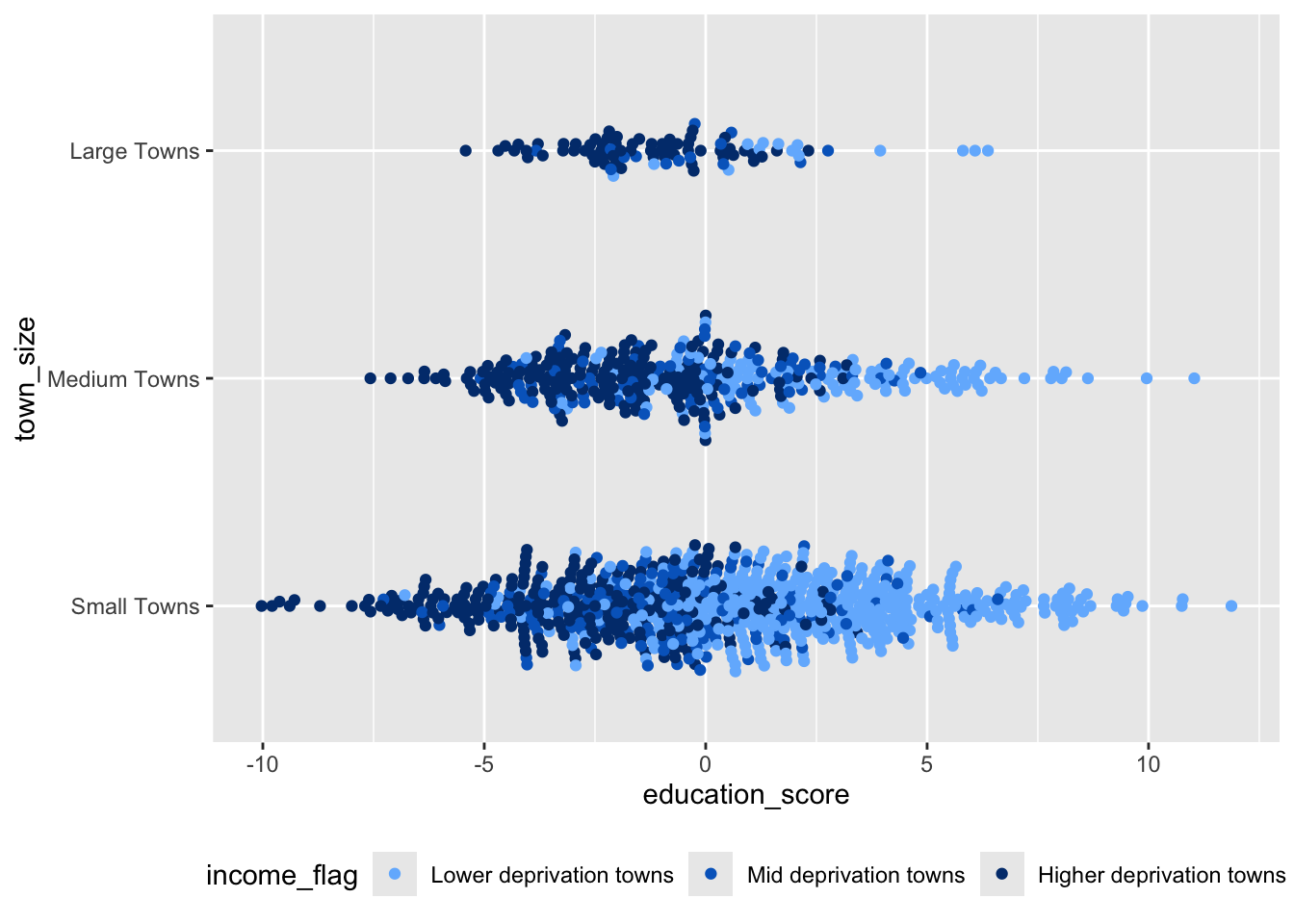
Conclusion
We were able to replicate the headline finding from the article, and the type of visualisation used. But we also identified area deprivation as an important (and likely a more important) determinant of education scores.