This TidyTuesday session investigated the funding of intrastructure steering committee grants from the R consortium over time, and was led by Kennedy Owuso-Afriyie.
Data loading
We looked at two options for loading the dataset: one using the tidytuesdayR package; the other linking to the url directly.
# A tibble: 85 × 7
    year group title                          funded proposed_by summary website
   <dbl> <dbl> <chr>                           <dbl> <chr>       <chr>   <chr>
 1  2023     1 The future of DBI (extension …  10000 "Kirill Mü… "This … <NA>
 2  2023     1 Secure TLS Communications for…  10000 "Charlie G… "The p… <NA>
 3  2023     1 volcalc: Calculate predicted …  12265 "Kristina … "This … <NA>
 4  2023     1 autotest: Automated testing o…   3000 "Mark Padg… "The p… <NA>
 5  2023     1 api2r: An R Package for Auto-…  15750 "Jon Harmo… "This … <NA>
 6  2022     2 D3po: R Package for Easy Inte…   8000 "Mauricio … "The D… <NA>
 7  2022     2 Tooling and Guidance for Tran…   8000 "Maëlle Sa… "Tooli… <NA>
 8  2022     2 Online Submission and Review …  22000 "Simon Urb… "The O… <NA>
 9  2022     2 Upgrading SatRdays Website Te…   6000 "Ben Ubah"  "The U… <NA>
10  2022     2 Building the “Spatial Data Sc…  25000 "Orhun Ayd… "The B… <NA>
# ℹ 75 more rows
Some questions we initially thought about asking:
Are there any keywords that stand out in the titles or summaries of awarded grants?
Have the funded amounts changed over time?
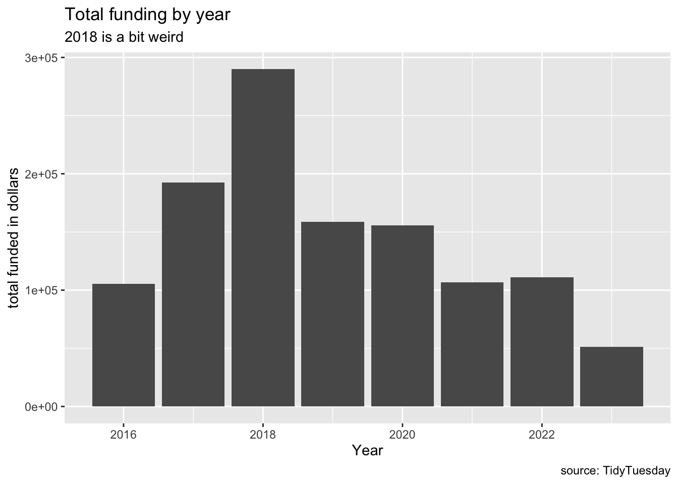
As a fairly new user to R, Kennedy focused on the second question, creating a bar plot of funding over time using ggplot. Meanwhile, Clarke and Clark investigated and proposed some approaches for addressing the first question.
Graph of funding over time
Code
funding_by_year <- isc_grants %>%group_by(year) %>%summarise(total_funded =sum(funded)) %>%ungroup()funding_by_year %>%ggplot(aes(x=year, y=total_funded)) +geom_col() +labs(x ="Year", y ="total funded in dollars",title ="Total funding by year",caption ="source: TidyTuesday",subtitle ="2018 is a bit weird" )
We discussed piping with the %>% operator, and the value this has for being able to develop code step-by-step in a way similar to human languages.
We said, when we see <- or ->, this should be read as ‘is assigned to’.
And we said, when we see the %>% (or |>) operator in a script, this should be read as, and then.
We noted how R can tell when it encounters an incomplete expression, and so doesn’t evaluate, just as when someone hears a sentence that ends ‘and then’, they know it’s not really the end of the sentence.
We also discussed how when making a graph, we should consider how objective or how subjective we should be when presenting the image to the viewer. This will depend on the audience. In our example, the x axis, y axis, title and caption labels are all just objective information. However the subtitle is more subjective, and so more our opinion rather than something no one could reasonably disagree with.
Tidy Text to get important key words
Brendan offered the following code chunk to explore the content of the free text summary field in the dataset:
Code
#install.packages("tidytext")#install.packages("SnowballC")library(tidytext)library(SnowballC) # for wordStemisc_grants |>unnest_tokens(word, summary) |>anti_join(get_stopwords()) |>mutate(stem =wordStem(word))
# A tibble: 6,242 × 8
    year group title                      funded proposed_by website word  stem
   <dbl> <dbl> <chr>                       <dbl> <chr>       <chr>   <chr> <chr>
 1  2023     1 The future of DBI (extens…  10000 Kirill Mül… <NA>    prop… prop…
 2  2023     1 The future of DBI (extens…  10000 Kirill Mül… <NA>    most… most…
 3  2023     1 The future of DBI (extens…  10000 Kirill Mül… <NA>    focu… focus
 4  2023     1 The future of DBI (extens…  10000 Kirill Mül… <NA>    main… main…
 5  2023     1 The future of DBI (extens…  10000 Kirill Mül… <NA>    supp… supp…
 6  2023     1 The future of DBI (extens…  10000 Kirill Mül… <NA>    dbi   dbi
 7  2023     1 The future of DBI (extens…  10000 Kirill Mül… <NA>    dbit… dbit…
 8  2023     1 The future of DBI (extens…  10000 Kirill Mül… <NA>    test  test
 9  2023     1 The future of DBI (extens…  10000 Kirill Mül… <NA>    suite suit
10  2023     1 The future of DBI (extens…  10000 Kirill Mül… <NA>    three three
# ℹ 6,232 more rows
This pulled out words (other than stopwords1) from the summary field, and identified the stem of these words. This potentially means the number of unique stems can be compared, rather than the number of unique words.
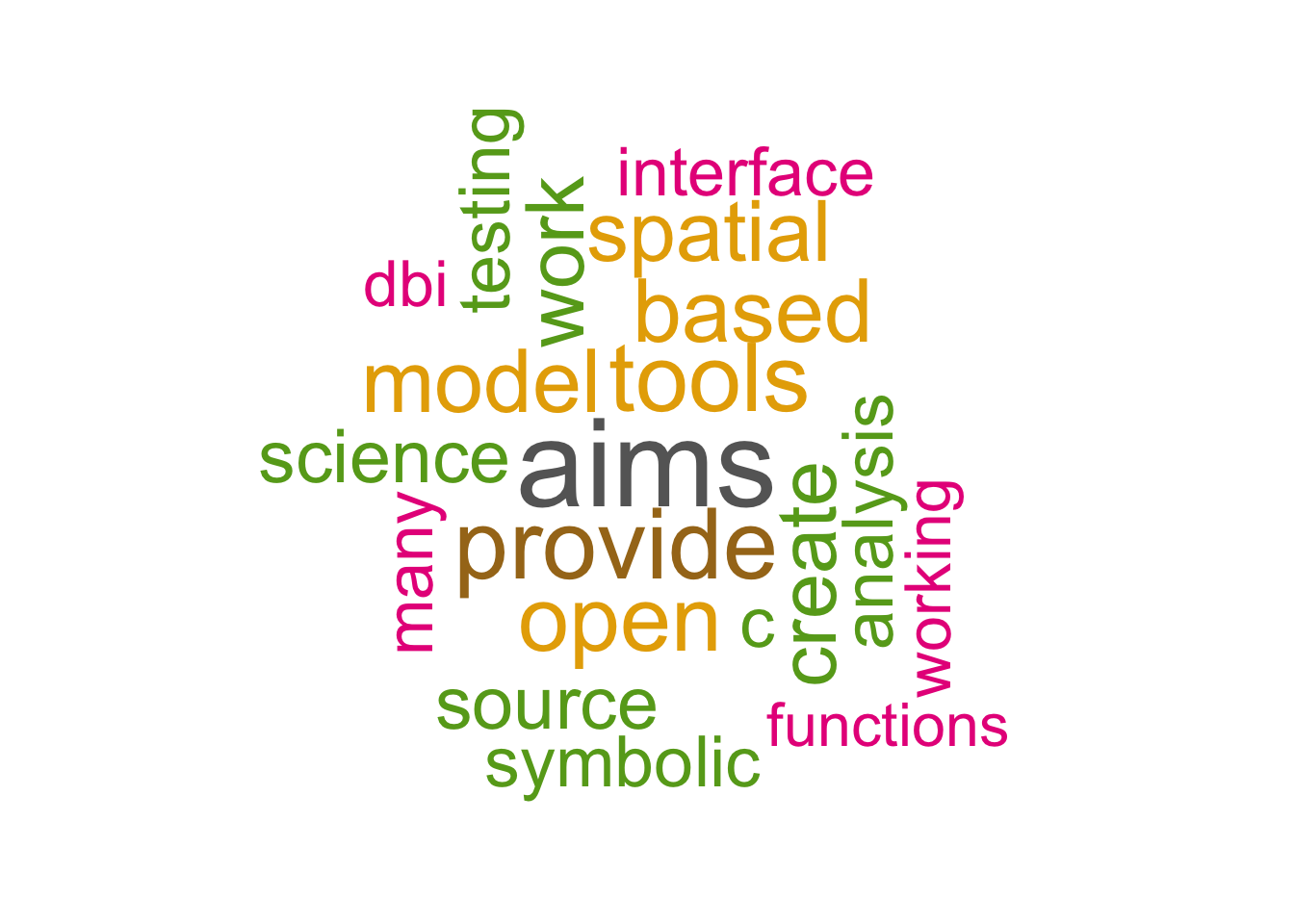
Antony suggested that, as the summaries are all about supporting a technical programing language, some additional words are also so common they should also be considered stopwords. He also produced a wordcloud visualisation showing the most common non-stopwords in the corpus of summary text”
Stop words are terms that are so common within sentences they don’t really add much unique information. They’re words like ‘and’, ‘the’, ‘an’, and so on.↩︎