Code
library(tidyverse)
library(broom)

tuesdata <- tidytuesdayR::tt_load(2024, week = 29)

ewf_appearances <- tuesdata$ewf_appearances
ewf_matches <- tuesdata$ewf_matches
ewf_standings <- tuesdata$ewf_standingsAfter a bit of a (in Jon’s view) dearth of interesting datasets within Tidy Tuesday, this week brought something worth looking at to the table: datasets on women’s football over the last few years, including changes in its popularity, as measured by attendance.
Kate led this session.
library(tidyverse)
library(broom)
tuesdata <- tidytuesdayR::tt_load(2024, week = 29)
ewf_appearances <- tuesdata$ewf_appearances
ewf_matches <- tuesdata$ewf_matches
ewf_standings <- tuesdata$ewf_standingsFirstly, we decided to look at growth attendance over time:
ewf_matches %>%
  group_by(season) %>%
  summarise(attendance = median(attendance, na.rm = TRUE)) %>%
  ggplot() +
  geom_col(aes(x = season, y = attendance)) +
  theme(axis.text.x = element_text(angle = 90))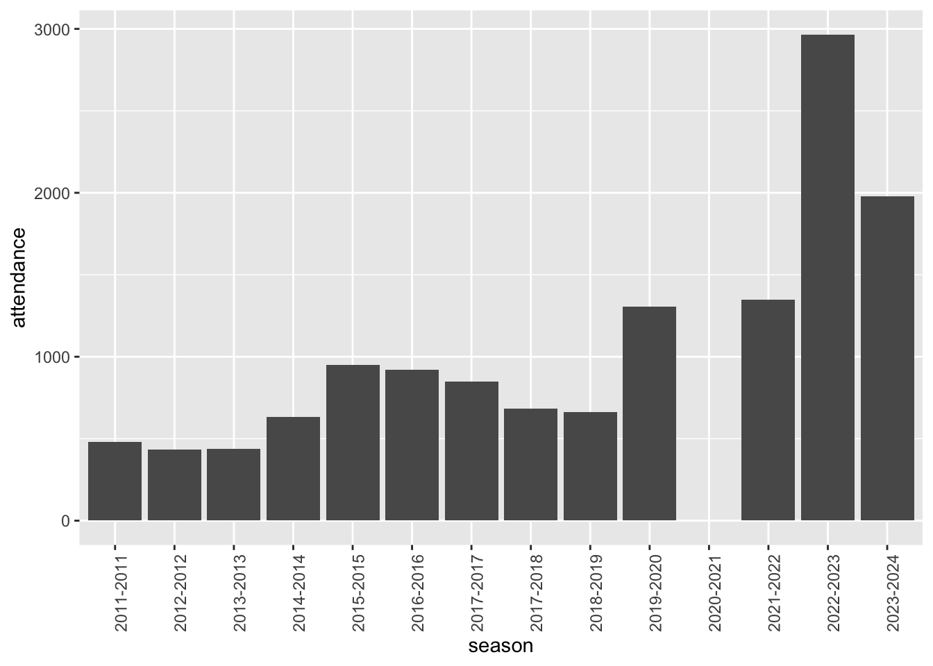
For some reason, there was no attendance in the 2020-2021 season. Definitely something unexpected that we should investigate further, as 2020 was a completely normal year in every way
What about trends in season, e.g. are the first matches more popular than the rest, much like the first episodes of TV series tend to be watched more than the rest of the series?
ewf_matches %>%
  group_by(season) %>%
  mutate(match_no = order(date)) %>%
  ggplot(aes(x = match_no, y = attendance, colour = season, group = season)) +
  geom_point() +
  facet_wrap(~ tier, scales = "free") +
  scale_y_log10()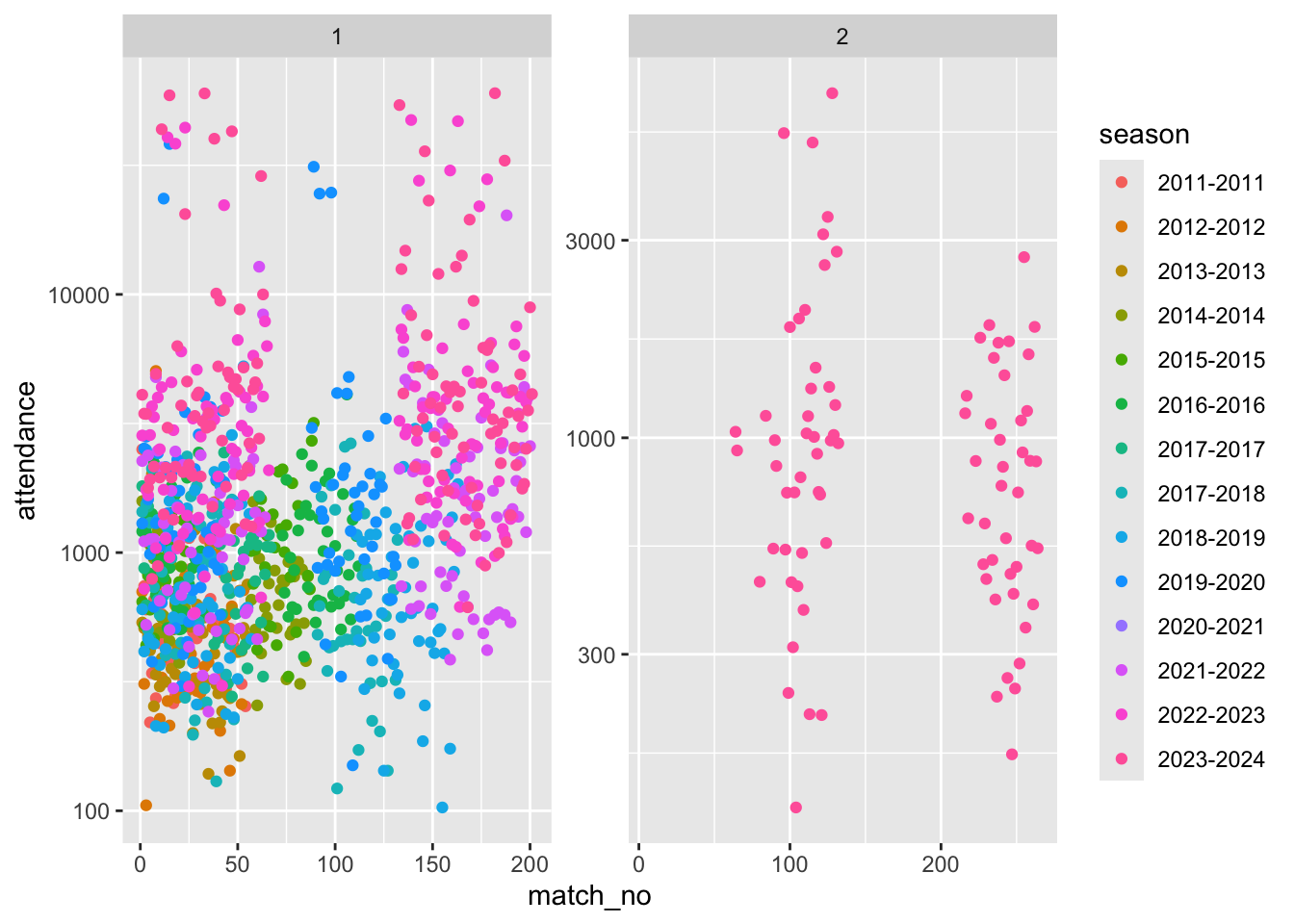
Note we used a log y scale as attendance seems to be very variable between matches. However we couldn’t see any obvious trend within season.
We also decided just to focus on tier 1
ewf_matches %>%
  filter(tier == 1) %>%
  group_by(season) %>%
  mutate(match_no = order(date)) %>%
  ggplot(aes(x = match_no, y = attendance, colour = season, group = season)) +
  geom_point() +
  scale_y_log10()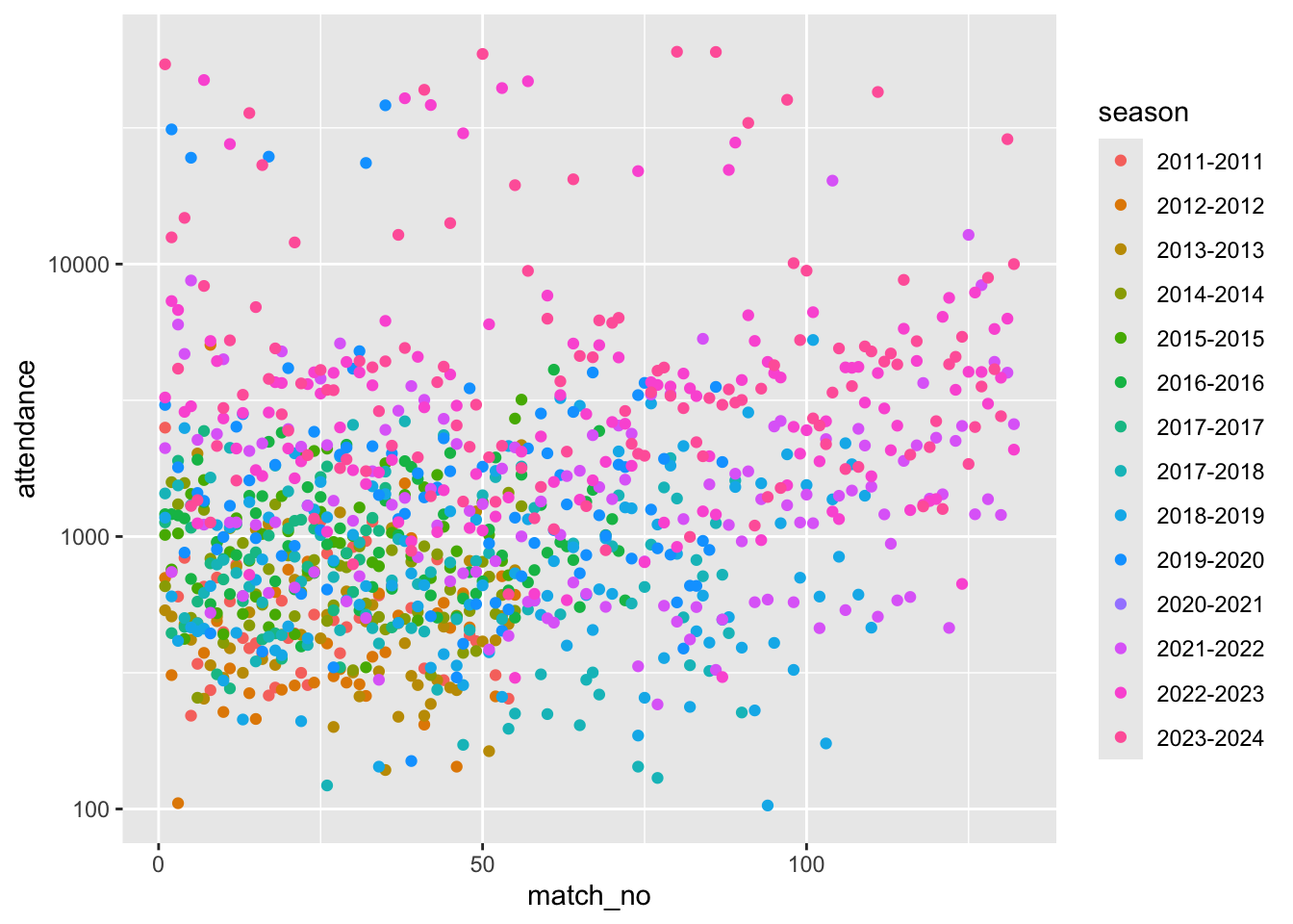
We then decided to try to model factors that could predict (log) attendance. First a model predicting log-attendance on home team id, match number, and season, but without interaction terms. And then a model with interaction terms:
ewf_matches %>%
  filter(tier == 1) %>%
  group_by(season) %>%
  mutate(match_no = order(date)) %>%
  lm(log10(attendance) ~ home_team_id + match_no + season, data = .) ->
  mod1

ewf_matches %>%
  filter(tier == 1) %>%
  group_by(season) %>%
  mutate(match_no = order(date)) %>%
  lm(log10(attendance) ~ home_team_id + match_no + season + season*match_no, data = .) ->
  mod2
How to compare? Well, as mod1 can be considered as a restricted version of mod2 (the interaction term coefficents set to 0) we can use ANOVA to see if the additional complexity of the unrestricted model, mod2, is ‘worth it’:
anova(mod2)Analysis of Variance Table
Response: log10(attendance)
Df Sum Sq Mean Sq F value Pr(>F)
home_team_id 17 63.340 3.7259 42.4441 < 2.2e-16 ***
match_no 1 4.241 4.2414 48.3166 6.604e-12 ***
season 12 56.470 4.7058 53.6073 < 2.2e-16 ***
match_no:season 12 1.508 0.1257 1.4314 0.1453
Residuals 982 86.203 0.0878
---
Signif. codes: 0 '***' 0.001 '**' 0.01 '*' 0.05 '.' 0.1 ' ' 1anova(mod1, mod2) # same as above but pulls out specific test that we are interested inAnalysis of Variance Table
Model 1: log10(attendance) ~ home_team_id + match_no + season
Model 2: log10(attendance) ~ home_team_id + match_no + season + season *
match_no
Res.Df RSS Df Sum of Sq F Pr(>F)
1 994 87.711
2 982 86.203 12 1.5079 1.4314 0.1453We concluded:
Interaction term not significant - proceed with mod1Now to look at the coefficients on mod1:
summary(mod1)
Call:
lm(formula = log10(attendance) ~ home_team_id + match_no + season,
    data = .)

Residuals:
     Min       1Q   Median       3Q      Max
-0.90496 -0.19277 -0.03661  0.14062  1.51043

Coefficients:
                      Estimate Std. Error t value Pr(>|t|)
(Intercept)          2.9890968  0.0541578  55.192  < 2e-16 ***
home_team_idT-002-T -0.2686225  0.0619191  -4.338 1.58e-05 ***
home_team_idT-003-T -0.3359697  0.0446896  -7.518 1.24e-13 ***
home_team_idT-005-T -0.2652441  0.0524152  -5.060 4.98e-07 ***
home_team_idT-006-T -0.2461753  0.0464112  -5.304 1.39e-07 ***
home_team_idT-008-T -0.0507938  0.0425091  -1.195 0.232413
home_team_idT-011-T -0.4073355  0.0693986  -5.870 5.95e-09 ***
home_team_idT-013-T -0.5394900  0.0448460 -12.030  < 2e-16 ***
home_team_idT-014-T -0.2734024  0.0619209  -4.415 1.12e-05 ***
home_team_idT-016-T -0.2675245  0.0598158  -4.472 8.62e-06 ***
home_team_idT-017-T -0.3209426  0.0440625  -7.284 6.60e-13 ***
home_team_idT-020-T -0.0394211  0.0447805  -0.880 0.378900
home_team_idT-021-T  0.0452529  0.0575592   0.786 0.431939
home_team_idT-023-T -0.4128162  0.0497442  -8.299 3.40e-16 ***
home_team_idT-027-T -0.4112510  0.0693942  -5.926 4.27e-09 ***
home_team_idT-028-T -0.3241747  0.0575895  -5.629 2.36e-08 ***
home_team_idT-030-T -0.3459956  0.0530576  -6.521 1.11e-10 ***
home_team_idT-031-T -0.3978321  0.0708242  -5.617 2.52e-08 ***
match_no            -0.0002474  0.0003161  -0.783 0.434030
season2012-2012     -0.0706150  0.0641552  -1.101 0.271298
season2013-2013     -0.0381315  0.0604345  -0.631 0.528215
season2014-2014      0.0752879  0.0611843   1.231 0.218797
season2015-2015      0.2112739  0.0626453   3.373 0.000774 ***
season2016-2016      0.2591016  0.0582373   4.449 9.60e-06 ***
season2017-2017      0.1782820  0.0691801   2.577 0.010107 *
season2017-2018      0.1231090  0.0579269   2.125 0.033812 *
season2018-2019      0.1606422  0.0562308   2.857 0.004368 **
season2019-2020      0.4160694  0.0578761   7.189 1.28e-12 ***
season2021-2022      0.3912164  0.0568712   6.879 1.06e-11 ***
season2022-2023      0.7350856  0.0570183  12.892  < 2e-16 ***
season2023-2024      0.8347182  0.0565907  14.750  < 2e-16 ***
---
Signif. codes:  0 '***' 0.001 '**' 0.01 '*' 0.05 '.' 0.1 ' ' 1

Residual standard error: 0.2971 on 994 degrees of freedom
  (178 observations deleted due to missingness)
Multiple R-squared:  0.5858,    Adjusted R-squared:  0.5733
F-statistic: 46.86 on 30 and 994 DF,  p-value: < 2.2e-16
We had some fun trying to find the most and least popular teams. The reference team, team 1, happens to be about the most popular team.
ewf_appearances %>%
  filter(season == "2023-2024") %>%
  select(team_id, team_name) %>%
  distinct() %>%
  arrange(team_id) |>
  view()
We thought we could do more to visualise the difference in apparent popularity between teams, producing some ‘tie fighter’ graphs (also known as blobograms, apparently)
tidy(mod1) %>%
  filter(str_detect(term, "home_team")) %>%
  mutate(term = str_remove(term, "home_team_id")) %>%
  ggplot() +
  geom_point(aes(x = estimate, y = term)) +
  geom_errorbarh(aes(xmin = estimate - 2*std.error, xmax = estimate + 2*std.error, y = term)) +
  geom_vline(aes(xintercept = 0), linetype = "dashed")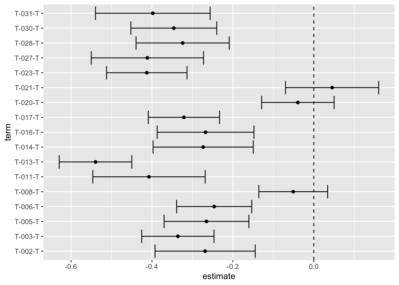
Poor old team 13! (Everton Women)
Compared with the reference team (Arsenal Women) only 3 teams looked similarly popular: team 8 (Chelsea Women), team 20 (Manchester City), and team 21 (Manchester United).
Then we decided to do the same kind of thing for season, which should showing growing popularity over time:
tidy(mod1) %>%
  filter(str_detect(term, "season")) %>%
  mutate(term = str_remove(term, "season")) %>%
  ggplot() +
  geom_point(aes(x = estimate, y = term)) +
  geom_errorbarh(aes(xmin = estimate - 2*std.error, xmax = estimate + 2*std.error, y = term)) +
  geom_vline(aes(xintercept = 0), linetype = "dashed")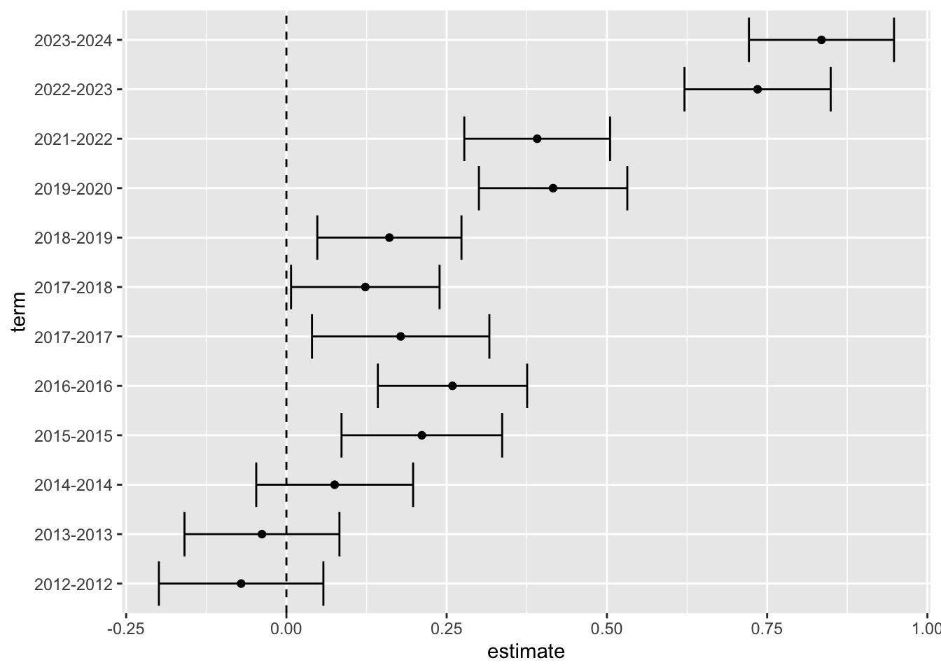
Up, up and away! (mostly…)
Some places to go: