This is part of a series of posts which introduce and discuss the implications of a general framework for thinking about statistical modelling. This framework is most clearly expressed in King et al. (2000).
Part 3: How to express a linear model as a generalised linear model
In the last part, we introduced two types of generalised linear models, with two types of transformation for the systematic component of the model, g(.), the logit transformation, and the identity transformation. This post will show how this framework is implemented in practice in R.
In R, there’s the lm function for linear models, and the glm function for generalised linear models.
I’ve argued previously that the standard linear regression is just a specific type of generalised linear model, one that makes use of an identity transformation I(.) for its systematic component g(.). Let’s now demonstrate that by producing the same model specification using both lm and glm.
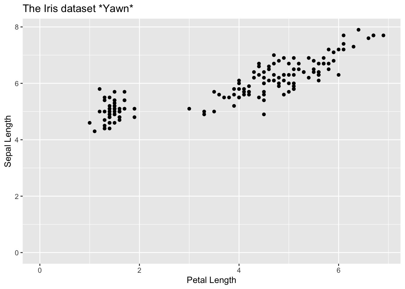
We can start by being painfully unimaginative and picking using one of R’s standard datasets
library(tidyverse)
── Attaching core tidyverse packages ──────────────────────── tidyverse 2.0.0 ──
✔ dplyr     1.1.4     ✔ readr     2.1.6
✔ forcats   1.0.1     ✔ stringr   1.6.0
✔ ggplot2   4.0.0     ✔ tibble    3.3.0
✔ lubridate 1.9.4     ✔ tidyr     1.3.1
✔ purrr     1.2.0
── Conflicts ────────────────────────────────────────── tidyverse_conflicts() ──
✖ dplyr::filter() masks stats::filter()
✖ dplyr::lag()    masks stats::lag()
ℹ Use the conflicted package (<http://conflicted.r-lib.org/>) to force all conflicts to become errors
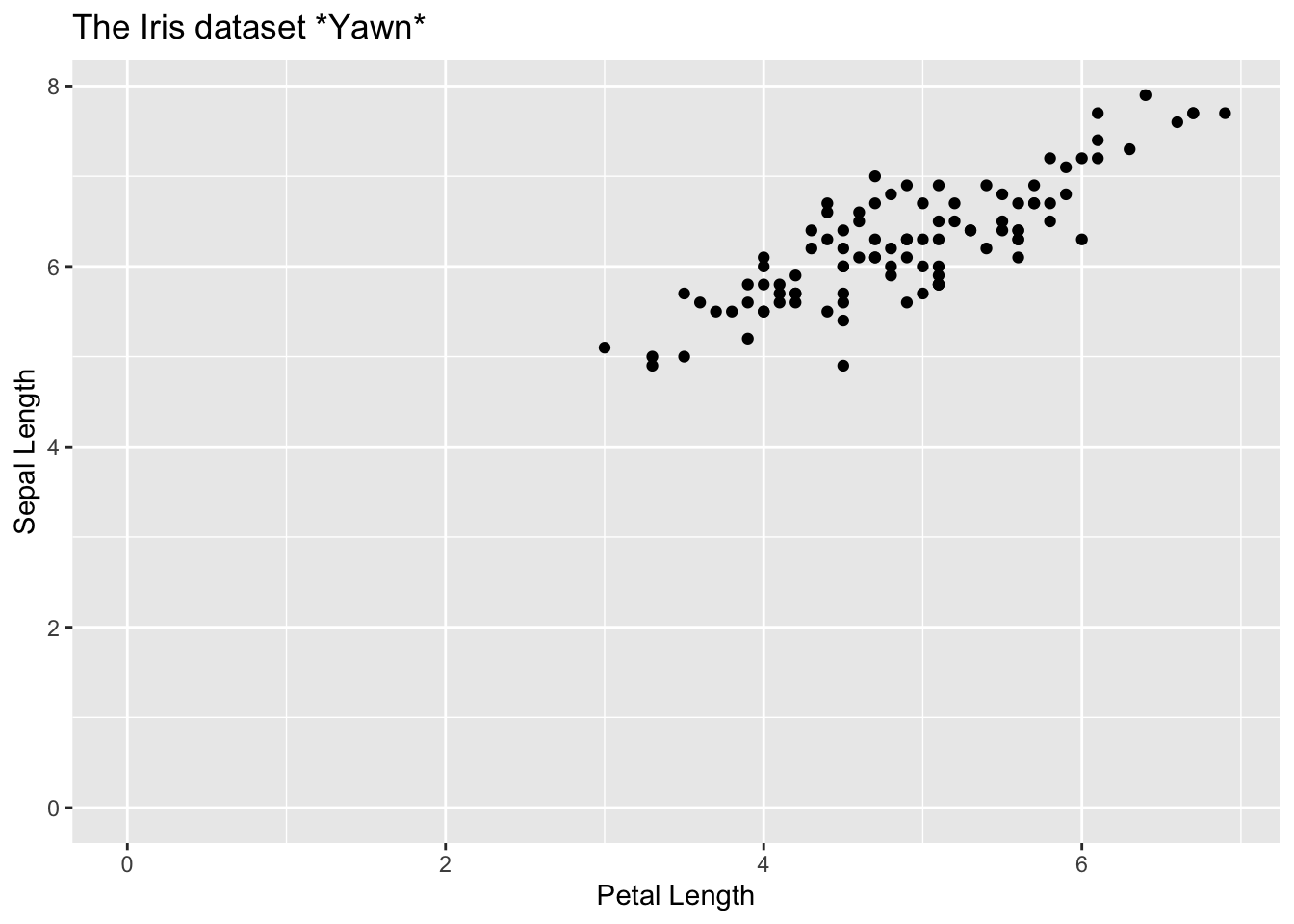
So, let’s make a linear regression just of this subset
iris_ss <- iris |>filter(Petal.Length >2.5)
We can produce the regression using lm as follows:
mod_lm <-lm(Sepal.Length ~ Petal.Length, data = iris_ss)
And we can use the summary function (which checks the type of mod_lm and evokes summary.lm implicitly) to get the following:
summary(mod_lm)
Call:
lm(formula = Sepal.Length ~ Petal.Length, data = iris_ss)

Residuals:
     Min       1Q   Median       3Q      Max
-1.09194 -0.26570  0.00761  0.21902  0.87502

Coefficients:
             Estimate Std. Error t value Pr(>|t|)
(Intercept)   2.99871    0.22593   13.27   <2e-16 ***
Petal.Length  0.66516    0.04542   14.64   <2e-16 ***
---
Signif. codes:  0 '***' 0.001 '**' 0.01 '*' 0.05 '.' 0.1 ' ' 1

Residual standard error: 0.3731 on 98 degrees of freedom
Multiple R-squared:  0.6864,    Adjusted R-squared:  0.6832
F-statistic: 214.5 on 1 and 98 DF,  p-value: < 2.2e-16
Woohoo! Three stars next to the Petal.Length coefficient! Definitely publishable!
To do the same using glm.
mod_glm <-glm(Sepal.Length ~ Petal.Length, data = iris_ss)
And we can use the summary function for this data too. In this case, summary evokes summary.glm because it knows the class of mod_glm contains glm.
summary(mod_glm)
Call:
glm(formula = Sepal.Length ~ Petal.Length, data = iris_ss)

Coefficients:
             Estimate Std. Error t value Pr(>|t|)
(Intercept)   2.99871    0.22593   13.27   <2e-16 ***
Petal.Length  0.66516    0.04542   14.64   <2e-16 ***
---
Signif. codes:  0 '***' 0.001 '**' 0.01 '*' 0.05 '.' 0.1 ' ' 1

(Dispersion parameter for gaussian family taken to be 0.1391962)

    Null deviance: 43.496  on 99  degrees of freedom
Residual deviance: 13.641  on 98  degrees of freedom
AIC: 90.58

Number of Fisher Scoring iterations: 2
So, the coefficients are exactly the same. But there’s also some additional information in the summary, including on the type of ‘family’ used. Why is this?
If we look at the help for glm we can see that, by default, the family argument is set to gaussian.
And if we delve a bit further into the help file, in the details about the family argument, it links to the family help page. The usage statement of the family help file is as follows:
Each family has a default link argument, and for this gaussian family, this link is the identity function.
We can also see that, for both the binomial and quasibinomial family, the default link is logit, which transforms all predictors onto a 0-1 scale, as shown in the last post.
So, by using the default family, the Gaussian family is selected, and by using the default Gaussian family member, the identity link is selected.
We can confirm this by setting the family and link explicitly, showing that we get the same results
mod_glm2 <-glm(Sepal.Length ~ Petal.Length, family =gaussian(link ="identity"), data = iris_ss)summary(mod_glm2)
Call:
glm(formula = Sepal.Length ~ Petal.Length, family = gaussian(link = "identity"),
    data = iris_ss)

Coefficients:
             Estimate Std. Error t value Pr(>|t|)
(Intercept)   2.99871    0.22593   13.27   <2e-16 ***
Petal.Length  0.66516    0.04542   14.64   <2e-16 ***
---
Signif. codes:  0 '***' 0.001 '**' 0.01 '*' 0.05 '.' 0.1 ' ' 1

(Dispersion parameter for gaussian family taken to be 0.1391962)

    Null deviance: 43.496  on 99  degrees of freedom
Residual deviance: 13.641  on 98  degrees of freedom
AIC: 90.58

Number of Fisher Scoring iterations: 2
It’s the same!
How do these terms used in the glm function, family and link, relate to the general framework in King et al. (2000)?
family is the stochastic component, f(.)
link is the systematic component, g(.)
They’re different terms, but it’s the same broad framework.
Linear models are just one type of general linear model!1
Coming up
In the next part of this series, we will delve into the differences between linear regression models and logistic regression models, with a focus on how to get meaningful effect estimates from both types of model.
References
King, Gary, Michael Tomz, and Jason Wittenberg. 2000. “Making the Most of Statistical Analyses: Improving Interpretation and Presentation.”American Journal of Political Science 44: 341355. http://gking.harvard.edu/files/abs/making-abs.shtml.
Footnotes
Note from Claude: For Python users, the equivalent functionality is available through multiple libraries. The statsmodels library most closely mirrors R’s approach: statsmodels.api.GLM(y, X, family=sm.families.Gaussian()) is equivalent to R’s glm(y ~ x, family=gaussian()). For production ML workflows, scikit-learn provides LinearRegression() and LogisticRegression() with simpler APIs but less statistical detail. The fast.ai course “Practical Deep Learning for Coders” demonstrates how these GLM concepts scale to deep learning, showing that even complex neural networks follow the same fit-predict-evaluate loop described in this series.↩︎