Part Nine: Answering questions with honest uncertainty: Expected values and Predicted values

Recap

The last eight posts in this series have taken us into some fairly arcane territory, including concepts like the use of link functions and statistical families within GLM, the likelihood theory of inference and its relation to Bayes’ Rule, and how models are fit in practice using optimisation algorithms. In the last couple of posts we showed how optim(), R’s standard optimisation function, can be used to recover not just the maximum likelihood (point) estimates of a series of parameters to be estimated, but also estimates of how much uncertainty there is about these estimates: both singularly, which gives rise to measures like standard errors, Z scores and P-values - the place where sadly all too many statistical analyses stop at; and jointly, through the calculation of the Hessian and corresponding variance-covariance matrix of uncertainty about the parameter vector.

In the last post, we showed how known uncertainty about the parameter values in the statistical model can be represented by using the point estimates \(\dot{\theta}\) and variance-covariance measure of uncertainty \(\Sigma\) can be used to produce a long series of plausible joint estimates of \(\tilde{\theta}\) (the parameter estimates with uncertainty) by passing the above as parameters to the multivariate normal distribution and taking repeated draws.

Aim

In this post, we’ll now, finally, show how this knowledge can be applied to do something with statistical models that ought to be done far more often: report on what King, Tomz, and Wittenberg (2000) calls quantities of interest, including predicted values, expected values, and first differences. Quantities of interest are not the direction and statistical significance (P-values) that many users of statistical models convince themselves matter, leading to the kind of mindless stargazing summaries of model outputs described in post four. Instead, they’re the kind of questions that someone, not trained to think that stargazing is satisfactory, might reasonably want answers to. These might include:

• What is the expected income of someone who completes course X in the five years after graduation? (Expected values)
• What is the expected range of incomes of someone who completes course X in the five years after graduation? (Predicted values)
• What is the expected difference in incomes between someone who completes course X, compared to course Y, in the five years after graduation? (First Differences)

In post four, we showed how to answer some of the questions of this form, for both standard linear regression and logistic regression. We showed that for linear regression such answers tend to come directly from the summary of coefficients, but that for logistic regression such answers tend to be both more ambiguous and dependent on other factors (such as gender of graduate, degree, ethnicity, age and so on), and require more processing in order to produce estimates for.

However, we previously produced only point estimates for these questions, and so in a sense misled the questioner with the apparent certainty of our estimates. We now know, from post eight, that we can use information about parameter uncertainty to produce parameter estimates \(\tilde{\theta}\) that do convey parameter uncertainty, and so we can do better than the point estimates alone to answer such questions in way that takes into account such uncertainty, with a range of values rather than a single value.

Method

Let’s make use of our toy dataset one last time, and go through the motions to produce the \(\tilde{\theta}\) draws we ended with on the last post:

Code

llNormal <- function(pars, y, X){
    beta <- pars[1:ncol(X)]
    sigma2 <- exp(pars[ncol(X)+1])
    -1/2 * (sum(log(sigma2) + (y - (X%*%beta))^2 / sigma2))
}

Code

# set a seed so runs are identical
set.seed(7)
# create a main predictor variable vector: -3 to 5 in increments of 1
x <- (-3):5
# Record the number of observations in x
N <- length(x)
# Create a response variable with variability
y <- 2.5 + 1.4 * x  + rnorm(N, mean = 0, sd = 0.5)

# bind x into a two column matrix whose first column is a vector of 1s (for the intercept)

X <- cbind(rep(1, N), x)
# Clean up names
colnames(X) <- NULL

Code

fuller_optim_output <- optim(
    par = c(0, 0, 0), 
    fn = llNormal,
    method = "BFGS",
    control = list(fnscale = -1),
    hessian = TRUE,
    y = y, 
    X = X
)

fuller_optim_output

$par
[1]  2.460675  1.375424 -1.336438

$value
[1] 1.51397

$counts
function gradient 
      80       36 

$convergence
[1] 0

$message
NULL

$hessian
              [,1]          [,2]          [,3]
[1,] -3.424917e+01 -3.424917e+01  2.727840e-05
[2,] -3.424917e+01 -2.625770e+02 -2.818257e-05
[3,]  2.727840e-05 -2.818257e-05 -4.500002e+00

Code

hess <- fuller_optim_output$hessian
inv_hess <- solve(-hess)
inv_hess

              [,1]          [,2]          [,3]
[1,]  3.357745e-02 -4.379668e-03  2.309709e-07
[2,] -4.379668e-03  4.379668e-03 -5.397790e-08
[3,]  2.309709e-07 -5.397790e-08  2.222221e-01

Code

point_estimates <- fuller_optim_output$par

vcov <- -solve(fuller_optim_output$hessian)
param_draws <- MASS::mvrnorm(
    n = 10000, 
    mu = point_estimates, 
    Sigma = vcov
)

colnames(param_draws) <- c(
    "beta0", "beta1", "eta"
)

Let’s now look at our toy data again, and decide on some specific questions to answer:

Code

library(tidyverse)
toy_df <- tibble(x = x, y = y)

toy_df |> 
    ggplot(aes(x = x, y = y)) + 
    geom_point()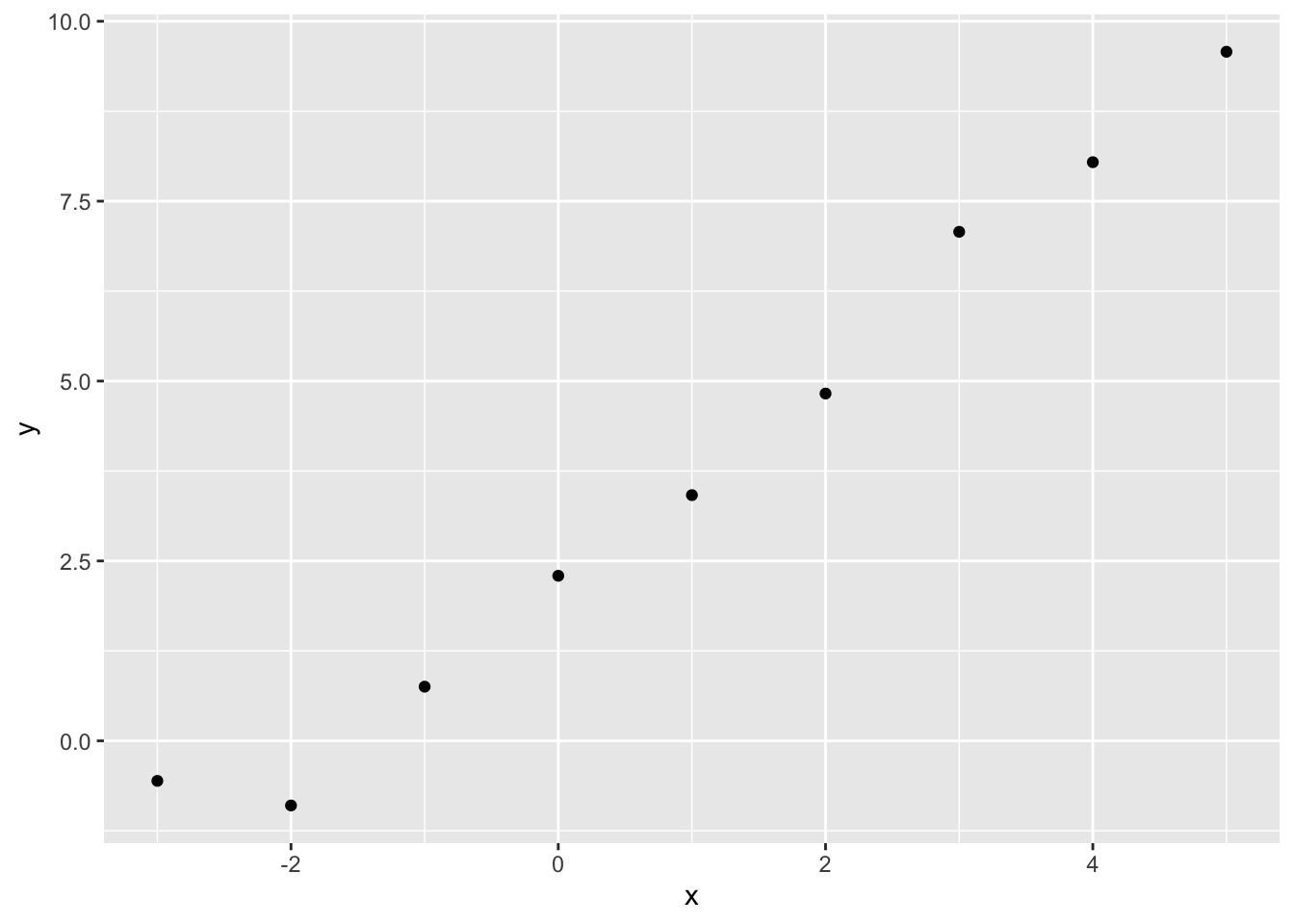 

Within the data itself, we have only supplied x and y values for whole numbers of x between -3 and 5. But we can use the model to produce estimates for non-integer values of x. Let’s try 2.5. For this single value of x, we can produce both predicted values and expected values, by passing the same value of x to each of the plausible estimates of \(\theta\) returned by the multivariate normal function above.

Code

candidate_x <- 2.5

Expected values

Here’s an example of estimating the expected value of y for x = 2.5 using loops and standard algebra:

Code

# Using standard algebra and loops
N <- nrow(param_draws)
expected_y_simpler <- vector("numeric", N)
for (i in 1:N){
    expected_y_simpler[i] <- param_draws[i, "beta0"] + candidate_x * param_draws[i, "beta1"]
}

head(expected_y_simpler)

[1] 6.004068 5.859547 6.121791 5.987509 5.767047 6.395820

We can see just from the first few values that each estimate is slightly different. Let’s order the values from lowest to highest, and find the range where 95% of values sit:

Code

ev_range <- quantile(expected_y_simpler,  probs = c(0.025, 0.500, 0.975)) 

ev_range

    2.5%      50%    97.5% 
5.505104 5.898148 6.291150 

The 95% interval is therefore between 5.51 and 6.29, with the median (similar but not quite the point estimate) being 5.90. Let’s plot this against the data:

Code

toy_df |> 
    ggplot(aes(x = x, y = y)) + 
    geom_point() + 
    annotate("point", x = candidate_x, y =  median(expected_y_simpler), size = 1.2, shape = 2, colour = "blue") + 
    annotate("segment", x = candidate_x, xend=candidate_x, y = ev_range[1], yend = ev_range[3], colour = "blue")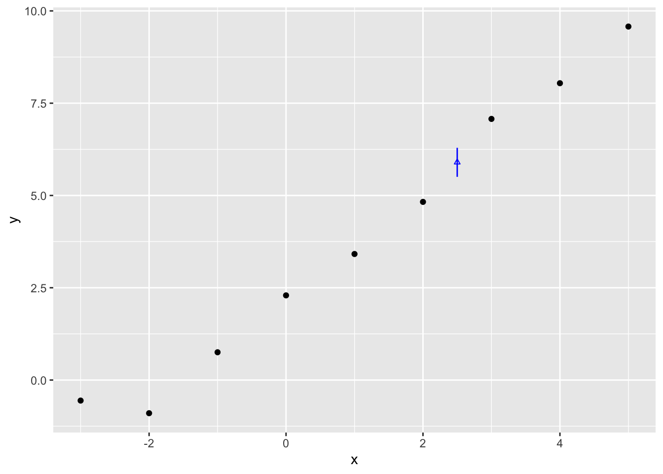

The vertical blue line therefore shows the range of estimates for \(Y|x=2.5\) that contain 95% of the expected values given the draws of \(\beta = \{\beta_0, \beta_1\}\) which we produced from the Multivariate Normal given the point estimates and Hessian from optim(). This is our estimated range for the expected value, not predicted value. What’s the difference?

Predicted values

One clue about the difference between expected value lies in the parameters from optim() we did and did not use: Whereas we have both point estimates and uncertainty estimates for the parameters \(\{\beta_0, \beta_1, \sigma^2\}\),¹ we only made use of the the two \(\beta\) parameters when producing this estimate.

Now let’s recall the general model formula, from the start of King, Tomz, and Wittenberg (2000), which we repeated for the first few posts in the series:

Stochastic Component

\[ Y_i \sim f(\theta_i, \alpha) \]

Systematic Component

\[ \theta_i = g(X_i, \beta) \]

The manual for Zelig, the (now defunct) R package that used to support analysis using this approach, states that for Normal Linear Regression these two components are resolved as follows:

Stochastic Component

\[ Y_i \sim Normal(\mu_i, \sigma^2) \]

Systematic Component

\[ \mu_i = x_i \beta \]

The page then goes onto state that the expected value, \(E(Y)\), is :

\[ E(Y) = \mu_i = x_i \beta \]

So, in this case, the expected value is the systematic component only, and does not involve the dispersion parameter in the stochastic component, which for normal linear regression is the \(\sigma^2\) term. That’s why we didn’t use estimates of \(\sigma^2\) when simulating the expected values.

But why is this? Well, it comes from the expectation operator, \(E(.)\). This operator means something like, return to me the value that would be expected if this experiment were performed an infinite number of times.

There are two types of uncertainty which give rise to variation in the predicted estimate: sampling uncertainty, and stochastic variation. In the expected value condition, this second source of variation falls to zero,² leaving only the influence of sampling uncertainty, as in uncertainty about the true value of the \(\beta\) parameters, remaining on uncertainty on the predicted outputs.

For predicted values, we therefore need to reintroduce stochastic variation as a source of variation in the range of estimates produced. Each \(\eta\) value we have implies a different \(\sigma^2\) value in the stochastic part of the equation, which we can then add onto the variation caused by parameter uncertainty alone:

Code

N <- nrow(param_draws)
predicted_y_simpler <- vector("numeric", N)
for (i in 1:N){
    predicted_y_simpler[i] <- param_draws[i, "beta0"] + candidate_x * param_draws[i, "beta1"] + 
        rnorm(
            1, mean = 0, 
            sd = sqrt(exp(param_draws[i, "eta"]))
        )
}

head(predicted_y_simpler)

[1] 4.802092 6.706397 7.073450 6.118750 6.757717 7.461254

Let’s now get the 95% prediction interval for the predicted values, and compare them with the expected values predicted interval earlier

Code

pv_range <- 
    quantile(
        predicted_y_simpler, 
        probs = c(0.025, 0.500, 0.975)
    )

pv_range

    2.5%      50%    97.5% 
4.766300 5.895763 7.055408 

So, whereas the median is similar to before, 5.90, the 95% interval is now from 4.77 to 7.06³. This compares with the 5.51 to 6.29 range for the expected values. Let’s now plot this predicted value range just as we did with the expected values:

Code

toy_df |> 
    ggplot(aes(x = x, y = y)) + 
    geom_point() + 
    annotate("point", x = candidate_x, y =  pv_range[2], size = 1.2, shape = 2, colour = "blue") + 
    annotate("segment", x = candidate_x, xend=candidate_x, y = pv_range[1], yend = pv_range[3], colour = "red")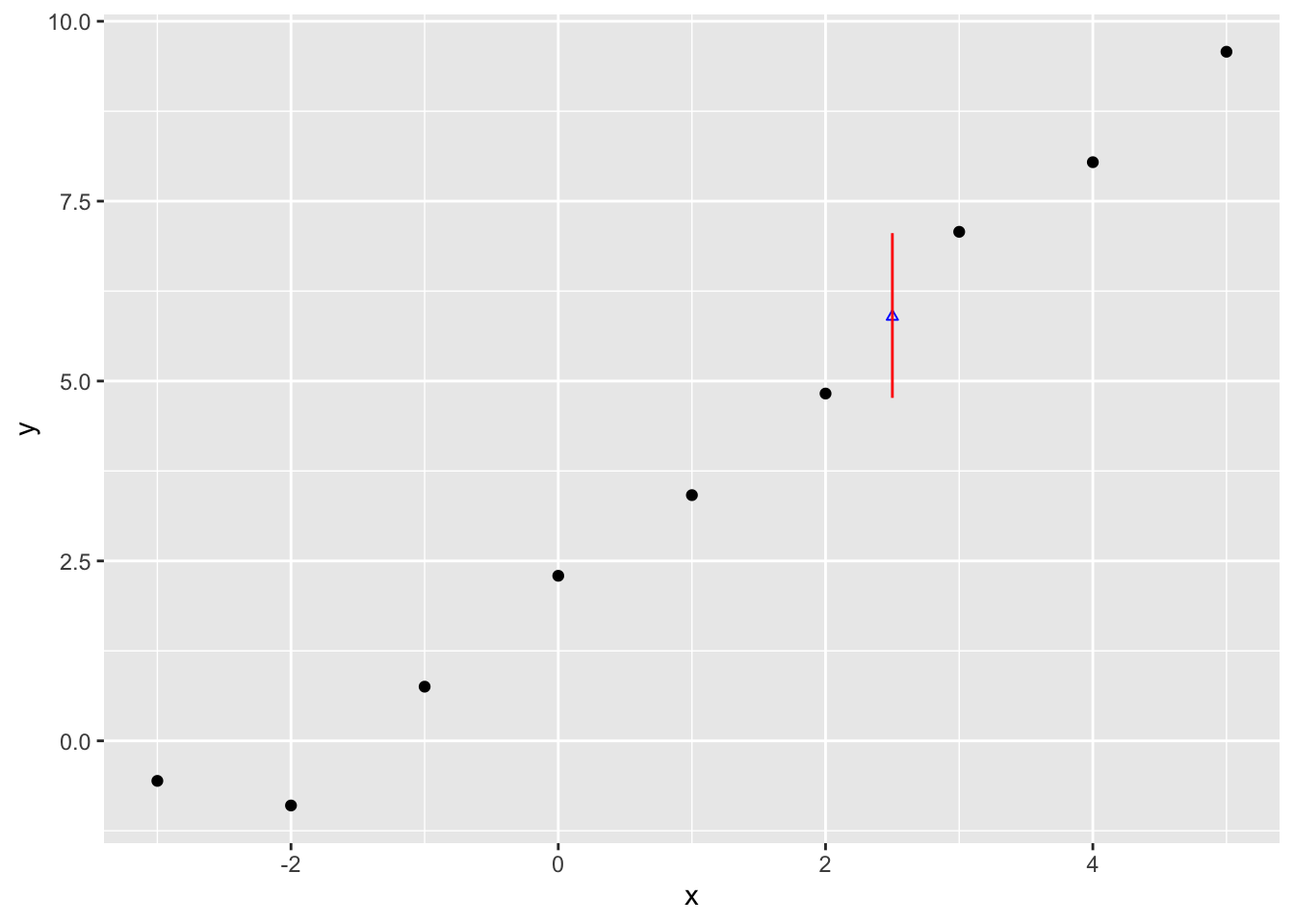

Clearly considerably wider.

Summary

This post is hopefully where our toy dataset, which we’ve been hauling with us since post five, can finally retire, happy in the knowledge that it’s taken us through some of the toughest parts of this blog series. The ideas developed over the last few posts can now finally be applied to answering some questions that are actually (or arguably) interesting!

Coming up

The next post covers the same kind of exercise we’ve performed for standard linear regression - specifying the likelihood function, and fitting it using optim() - but for logistic regression instead. This same kind of exercise could be repeated for all kinds of other model types. But hopefully this one additional example is sufficient.

References

King, Gary, Michael Tomz, and Jason Wittenberg. 2000. “Making the Most of Statistical Analyses: Improving Interpretation and Presentation.” American Journal of Political Science 44: 341355. http://gking.harvard.edu/files/abs/making-abs.shtml.

Footnotes

1. Where \(\sigma^2\) is from \(\eta\) and we defined \(e^{\eta} = \sigma^2\), a transformation which allowed optim() to search over an unbounded rather than bounded real number line

2. It can be easier to see this by using the more conventional way of expressing Normal linear regression: \(Y_i = x_i \beta + \epsilon\), where \(\epsilon \sim Normal(0, \sigma^2)\). The expectation is therefore \(E(Y_i) = E( x_i \beta + \epsilon ) = E(x_i \beta) + E(\epsilon)\). For the first part of this equation, \(E(x_i \beta) = x_i \beta\), because the systematic component is always the same value, no matter how many times a draw is taken from the model. And for the second part, \(E(\epsilon) = 0\), because Normal distributions are symmetrical around their central value over the long term: on average, every large positive value drawn from this distribution will become cancelled out by an equally large negative value, meaning the expected value returned by the distribution is zero. Hence, \(E(Y) = x_i \beta\).

3. Because these estimates depend on random variation, these intervals may be slightly different to two decimal places than the values I’m quoting here.