Part Nineteen: Time Series: Introduction and Autoregression
statistics
time series
Author
Jon Minton
Published
April 21, 2024
Introduction
A few weeks ago, I polled both LinkedIn and (what’s left of) Twitter for statistical topics to cover next in this series. By a small to moderate margin, time series came out on top. So, after a longer-than-usual delay, here’s an introduction to time series modelling.
Time Series: An exception that proves the rule?
Throughout this series I’ve returned many times to the same ‘mother formula’ for a generalised linear model:
Stochastic Component
\[
Y_i \sim f(\theta_i, \alpha)
\]
Systematic Component
\[
\theta_i = g(X_i, \beta)
\]
So, we have a system that takes a series of inputs, \(X\), and returns an output, \(Y\), and we have two sets of parameters, \(\beta\) in \(g(.)\) and \(\alpha\) in \(f(.)\), which are calibrated based on the discrepancy between what the model predicted output \(Y\) and the observed output \(y\).
There are two important things to note: Firstly, that the choice of parts of the data go into the inputs \(X\) and the output(s) \(Y\) is ultimately our own. A statistical model won’t ‘know’ when we’re trying to predict the cause of something based on its effect, for example. Secondly, that although the choice of input and output for the model are ultimately arbitrary, they cannot be the same. i.e., we cannot do this:
\[
Y_i \sim f(\theta_i, \alpha)
\]
\[
\theta_i = g(Y_i, \beta)
\]
This would be the model calibration equivalent of telling a dog to chase, or a snake to eat, its own tail. It doesn’t make sense, and so the parameter values involved cannot be calculated.
For time series data, however, this might appear to be a fundamental problem, given our observations may comprise only of ‘outcomes’, which look like they should be in the output slot of the formulae, rather than determinants, which look like they should be in the input slot of the formulae. i.e. we might have data that looks as follows:
\(i\)
\(Y_{T-2}\)
\(Y_{T-1}\)
\(Y_{T}\)
1
4.8
5.0
4.9
2
3.7
4.1
4.3
3
4.3
4.1
4.3
Where \(T\) indicates an index time period, and \(T-k\) a fixed difference in time ahead of or behind the index time period. For example, \(T\) might be 2019, \(T-1\) might be 2018, \(T-2\) might be 2017, and so on.
Additionally, for some time series data, the dataset will be much more wide than long, perhaps with just a single observed unit, observed at many different time points:
\(i\)
\(Y_{T-5}\)
\(Y_{T-4}\)
\(Y_{T-3}\)
\(Y_{T-2}\)
\(Y_{T-1}\)
\(Y_{T}\)
1
3.9
5.1
4.6
4.8
5.0
4.9
Given all values are ‘outcomes’, where’s the candidate for an ‘input’ to the model, i.e. something we should consider putting into \(X\)?
Doesn’t the lack of an \(X\) mean time series is an exception to the ‘rule’ about what a statistical model looks like, and so everything we’ve learned so far is no longer relevant?
The answer to the second question is no. Let’s look at why.
Autoregression
Instead of looking at the data in the wide format above, let’s instead rearrange it in long format, so the time variable is indexed in its own column:
# A tibble: 6 × 3
      i     t     y
  <dbl> <dbl> <dbl>
1     1  2008   3.9
2     1  2009   5.1
3     1  2010   4.6
4     1  2011   4.8
5     1  2012   5
6     1  2013   4.9
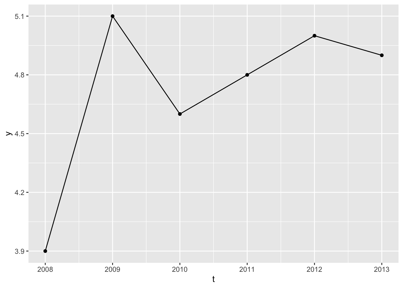
As there’s only one type of observational unit, \(i=1\) in all cases, there’s no variation in this variable, so it can’t provide any information in a model. Let’s look at the series and think some more:
Code
df |>ggplot(aes(t, y)) +geom_line() +geom_point()
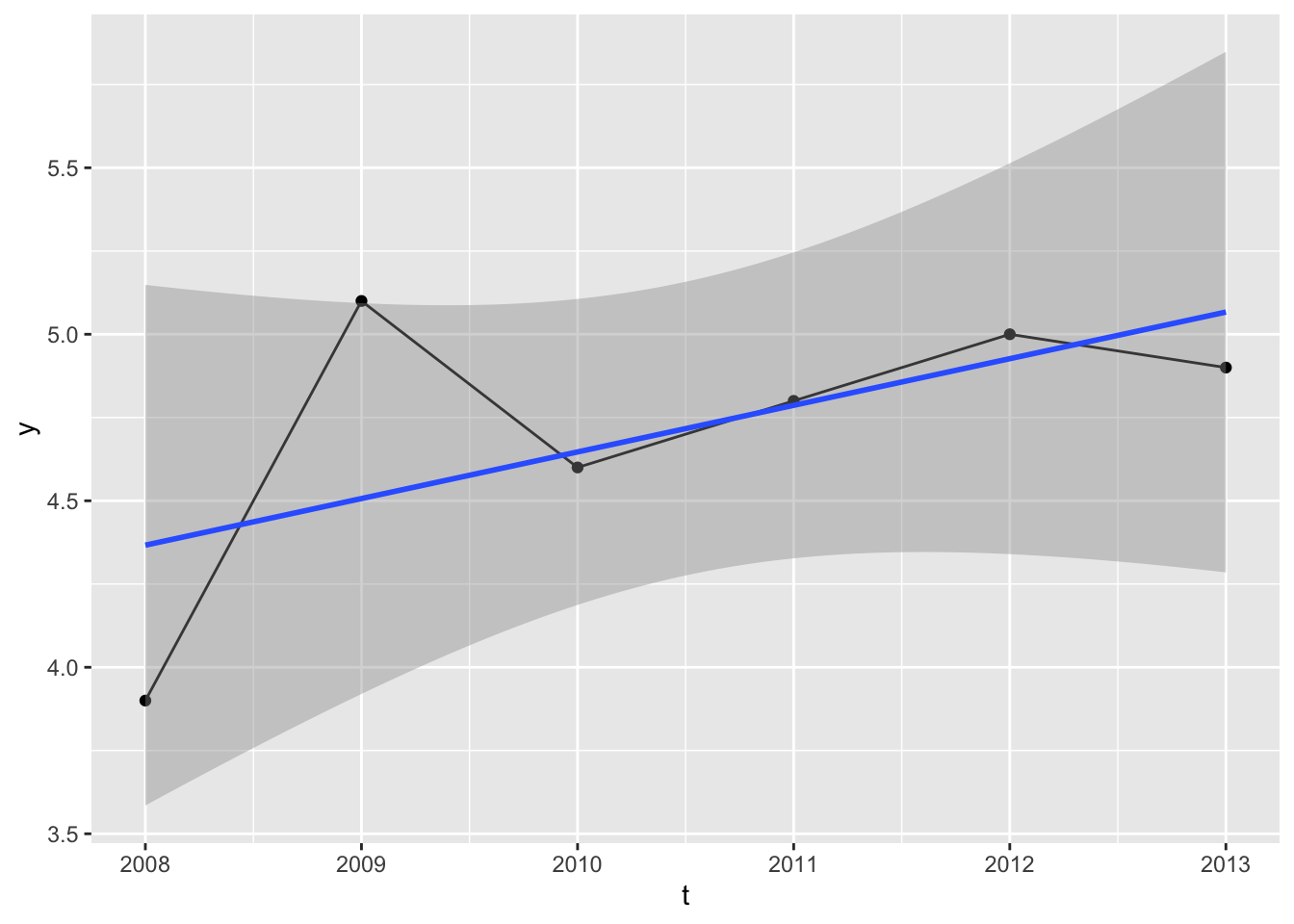
We could, of course, regress the outcome against time:
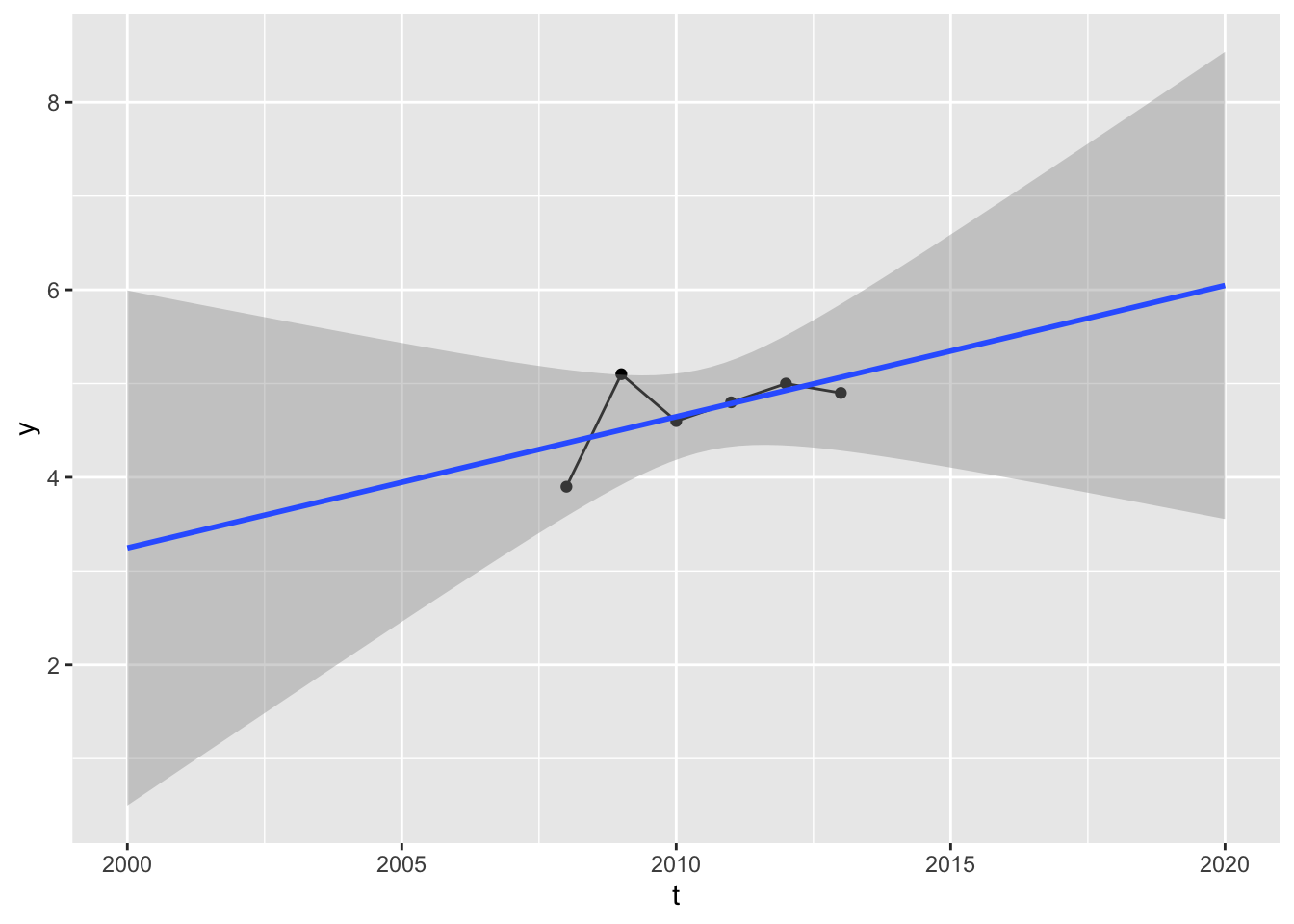
Is this reasonable? It depends on the context. We obviously don’t have that many observations, but the regression slope appears to have a positive gradient, meaning values projected into the future will likely be higher than the observed values, and values projected into the past will likely have lower than the observed values.
Maybe this kind of extrapolation is reasonable. Maybe it’s not. As usual it depends on context. Although it’s a model including time as a predictor, it’s not actually a time series model. Here’s an example of a time series model:
Code
lm_ts_ar0 <-lm(y ~1, data = df)summary(lm_ts_ar0)
Call:
lm(formula = y ~ 1, data = df)

Residuals:
       1        2        3        4        5        6
-0.81667  0.38333 -0.11667  0.08333  0.28333  0.18333

Coefficients:
            Estimate Std. Error t value Pr(>|t|)
(Intercept)   4.7167     0.1778   26.53 1.42e-06 ***
---
Signif. codes:  0 '***' 0.001 '**' 0.01 '*' 0.05 '.' 0.1 ' ' 1

Residual standard error: 0.4355 on 5 degrees of freedom
This is an example of a time series model, even though it doesn’t have a time component on the predictor side. In fact, it doesn’t have anything as a predictor. Its formula is y ~ 1, meaning there’s just an intercept term. It’s saying “assume new values are just like old values: all just drawn from the same normal distribution”.
I called this model ar0. Why? Well, let’s look at the following:
Call:
lm(formula = y ~ y_lag1, data = .)

Residuals:
        2         3         4         5         6
-0.005066 -0.158811 -0.103084  0.154626  0.112335

Coefficients:
            Estimate Std. Error t value Pr(>|t|)
(Intercept)   6.2304     0.7661   8.132  0.00389 **
y_lag1       -0.2885     0.1630  -1.770  0.17489
---
Signif. codes:  0 '***' 0.001 '**' 0.01 '*' 0.05 '.' 0.1 ' ' 1

Residual standard error: 0.1554 on 3 degrees of freedom
  (1 observation deleted due to missingness)
Multiple R-squared:  0.5108,    Adjusted R-squared:  0.3477
F-statistic: 3.133 on 1 and 3 DF,  p-value: 0.1749
For this model, I included one new predictor: y_lag1. For this, I created a new column in the dataset:
Code
df |>arrange(t) |>mutate(y_lag1 =lag(y, 1))
# A tibble: 6 × 4
      i     t     y y_lag1
  <dbl> <dbl> <dbl>  <dbl>
1     1  2008   3.9   NA
2     1  2009   5.1    3.9
3     1  2010   4.6    5.1
4     1  2011   4.8    4.6
5     1  2012   5      4.8
6     1  2013   4.9    5
The lag() operator takes a column and a lag term parameter, in this case 11. For each row, the value of y_lag1 is the value of y one row above. 2
The first simple model was called AR0, and the second AR1. So what does AR stand for?
If you’re paying attention to the section title, you already have the answer. It means autoregressive. The AR1 model is the simplest type of autoregressive model, by which I don’t mean this is a type of regression model that formulates itself, but do mean it includes its own past states (at time T-1) as predictors of its current state (at time T).
And what does \(T\) and \(T-1\) refer to in the above? Well, for row 6 \(T\) refers to \(t\), which is 2013; and so \(T-1\) refers to 2012. But for row 5 \(T\) refers to 2012, so \(T-1\) refers to 2011. This continues back to row 2, where \(T\) is 2009 so \(T-1\) must be 2008. (The first row doesn’t have a value for y_lag1, so can’t be included in the regression).
Isn’t this a bit weird, however? After all, we only have one real observational unit, \(i\), but for the AR1 model we’re using values from this unit five times. Doesn’t this violate some kind of rule or expectation required for model outputs to be legitimate?
Well, it might. A common shorthand when describing the assumptions that we make when applying statistical models is \(IID\), which stands for ‘independent and identically distributed’. As with many unimaginative discussions of statistics, we can illustrate something that satifies both of these properties, independent and identically distributed by looking at some coin flips:
The above series of coin flips is identically distributed because the order in which the flips occur doesn’t matter to the value generated. The dataframe could be permutated in any order and it wouldn’t matter to the data generation process at all. The series is independent because the probability of getting, say, a sequence of three heads is just the product of getting one head, three times, i.e. i.e. \(\frac{1}{2} \frac{1}{2} \frac{1}{2}\) or \([\frac{1}{2}]^{3}\). Without going into too much detail, both of these assumptions are necessary to make in order for likelihood estimation, which relies on multiplying sequences of numbers 3 to ‘work’.
The central assumption and hope with an autoregressive model specification is that, conditional on the autoregressive terms being included on the predictor side of the model, the data can assumed to have been generated from an IID data generating process (DGP).
The intuition behind this is something like the following: say you wanted to know if I’ll have the flu tomorrow. It would obviously be useful to know if I have the flu today, because symptoms don’t change very quickly. 4 Maybe it would also be good to know if I had the flu yesterday too, maybe even two days ago as well. But would it be good to know if I had the flu two weeks ago, or five weeks ago? Probably not. At some point, i.e. some number of lag terms from a given time, more historical data stops being informative. i.e., beyond a certain number of lag periods, the data series can be assumed to be IID (hopefully).
When building autoregressive models, it is common to look at a range of specifications, each including different numbers of lag terms. I.e. we can build a series of AR specification models as follows:
AR(0): \(Y_T \sim 1\)
AR(1): \(Y_T \sim Y_{T-1}\)
AR(2): \(Y_T \sim Y_{T-1} + Y_{T-2}\)
AR(3): \(Y_T \sim Y_{T-1} + Y_{T-2} + Y_{T-3}\)
And so on. Each successive AR(.) model contains more terms than the last, so is a more complicated and data hungry model than the previous one. We should already by this point in the series be familiar with standard approaches for trying to find the best trade off between model complexity and model fit. The above models are in a sense nested, so for example F-tests can be used to compare these models. Another approach, which ‘works’ for both nested and non-nested model specifications, is AIC, and indeed this is commonly used to select the ‘best’ number of autoregressive terms to include.
For future reference, the number of AR terms is commonly denoted with the letter ‘p’, meaning that if p is 3, for example, then we are talking about an AR(3) model specification.
Summing up
The other important thing to note is that autoregression is a way of fitting time series data within the two component ‘mother formulae’ at the start of this post (and many others), by operating on the systematic component of the model framework, \(g(.)\). At this stage, nothing unusual is happening with the stochastic component of the model framework \(f(.)\).
With autoregression, denoted by the formula shorthand \(AR(.)\) and the parameter shorthand \(p\), we now have one of the three main tools in the modeller’s toolkit for handling time series data.
Coming up
In the next post in this mini-series, we’ll start to look at the other two main components of time series modelling, integration and moving averages, before looking at how they’re combined and applied in a general model specification called ARIMA.
Footnotes
Which is also the default, so not strictly necessary this time.↩︎
Two further things to note: Firstly, that if there were more than one observational unit i then the data frame should be grouped by the observational unit, then arranged by time. Secondly, that because the first time unit has no time unit, its lagged value is necessarily missing, hence NA.↩︎
Or equivalently and more commonly summing up the log of these numbers↩︎
This is in some ways a bad example, as influenza is of course highly seasonal, and one flu episode may be negatively predictive of another flu episode in the same season. But I’m going with it for now…↩︎