In the last part of this series, I discussed why time series data are both a bit dissimilar to many other types of data we try to model, and also ‘one weird trick’ - autoregression - which allows the standard generalised linear model ‘chasis’ - that two part equation - to be used with time series data.
Within the last part, I said autoregression was just one of three common tools used for working with time series data, with the other two being integration and moving averages. Let’s now cover those two remaining tools:
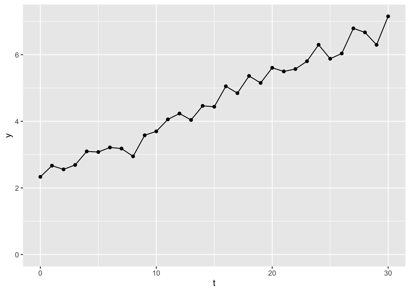
This time series data is an example of a non-stationary time series. This term means that its value drifts in a particular direction over time. In this case, upwards, meaning values towards the end of the series tend to be higher than values towards the start of the series.
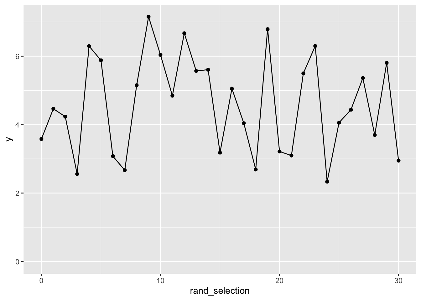
What this drift means is that the order of the observations matters, i.e. if we looked at the same observations, but in a random order, we wouldn’t see something that looks similar to what we’re seeing here.
As it’s clear the order of the sequence matters, the standard simplifying assumptions for statistical models of IID (independent and identically distributed) does not hold, so the extent to which observations from the same time series dataset can be treated like new pieces of information for the model is doubtful. We need a way of making the observations that go into the model (though not necessarily what we do with the model after fitting it) more similar to each other, so these observations can be treated as IID. How do we do this?
The answer is something that’s blindingly obvious in retrospect. We can transform the data that goes into the model by taking the differences between consecutive values. So, if the first ten values of our dataset look like this:
So, as with autoregression (AR), with integration we’ve arranged the data in order, then used the lag operator. The difference between the use of lagging as a tool for AR, and lagging as a tool for integration (I), is that, whereas for autoregression, we’re using lagging to construct one or more variables to use as predictor terms for the model, within integration we’re using lagging to construct new variables for use in either the response or the predictor sides of the model equation.
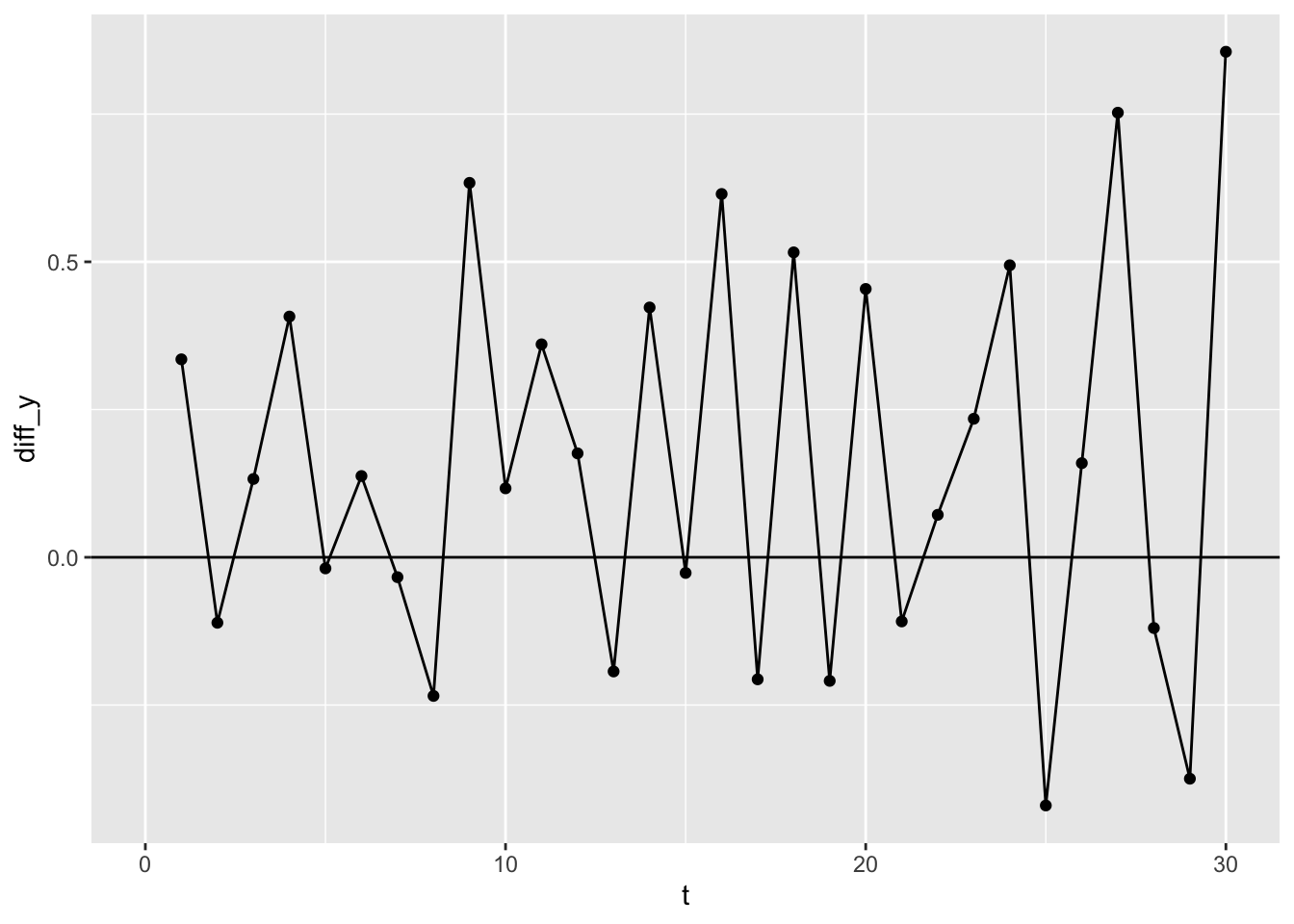
In the above I’ve added a reference line at y=0. Note that the average of this series appears to be above the zero line. Let’s check this assumption:
Code
dy <- df |>arrange(t) |>mutate(diff_y = y -lag(y, 1)) |>pull(diff_y) print(paste0("The mean dy is ", mean(dy, na.rm =TRUE) |>round(2)))
[1] "The mean dy is 0.16"
Code
print(paste0("The corresponding SE is ", (sd(dy, na.rm=TRUE) /sqrt(length(dy)-1)) |>round(2)))
[1] "The corresponding SE is 0.06"
This mean value of the differences values, \(dy\), is about 0.16. This is the intercept of the differenced data. As we made up the original data, we also know that its slope is 0.15, i.e. except for estimation uncertainty, the intercept of the differenced data is the slope of the original data. 1
Importantly, when it comes to time series, whereas our original data were not stationary, our differenced data are. This means they are more likely to meet the IID conditions, including that the order of observations no longer really matters as to its value.
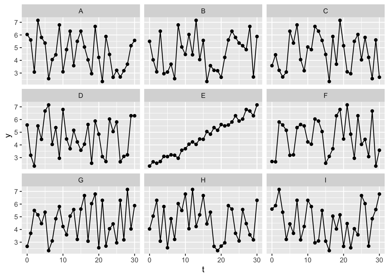
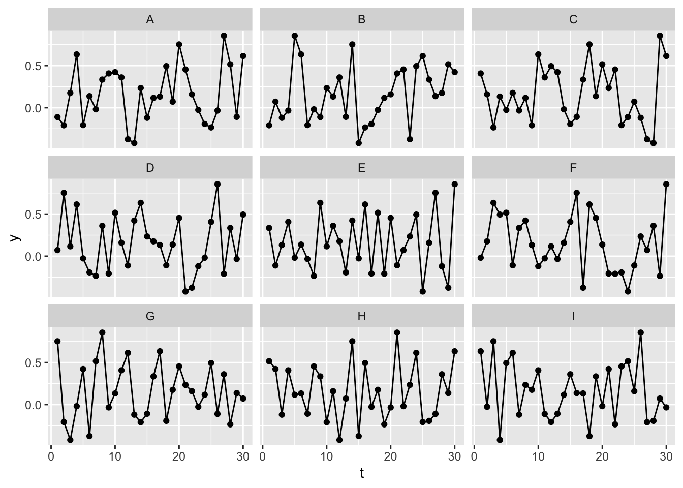
One way of demonstrating this is with a statistical identity parade.
Here are nine versions of the undifferenced data, eight of which have been randomly shuffled. Can you tell which is the original, unshuffled data?
Here it seems fairly obvious which dataset is the original, unshuffled version of the data, again illustrating that the original time series are not IID, and not a stationary series.
By contrast, let’s repeat the same exercise with the differenced data:
Here it’s much less obvious which of the series is the original series, rather than a permuted/shuffled version of the same series. This should give some reassurance that, after differencing, the data are now IID.
Why is integration called integration not differencing?
In the above we have performed what in time series parlance would be called an I(1) operation, differencing the data once. But why is this referred to as integration, when we’re doing the opposite?
Well, when it comes to transforming the time series data into something with IID properties, we are differentiating rather than integrating. But the flip side of this is that, if using model outputs based on differenced data for forecasting, we have to sum up (i.e. integrate) the values we generate in the order in which we generate them. So, the model works on the differenced data, but model forecasts work by integrating the random variables generated by the model working on the differenced data.
Let’s explore what this means in practice. Let’s generate 10 new values from a model calibrated on the mean and standard deviation of the differenced data:
Code
new_draws <-rnorm(10, mean =mean(d_df$y, na.rm =TRUE),sd =sd(d_df$y, na.rm =TRUE))new_draws
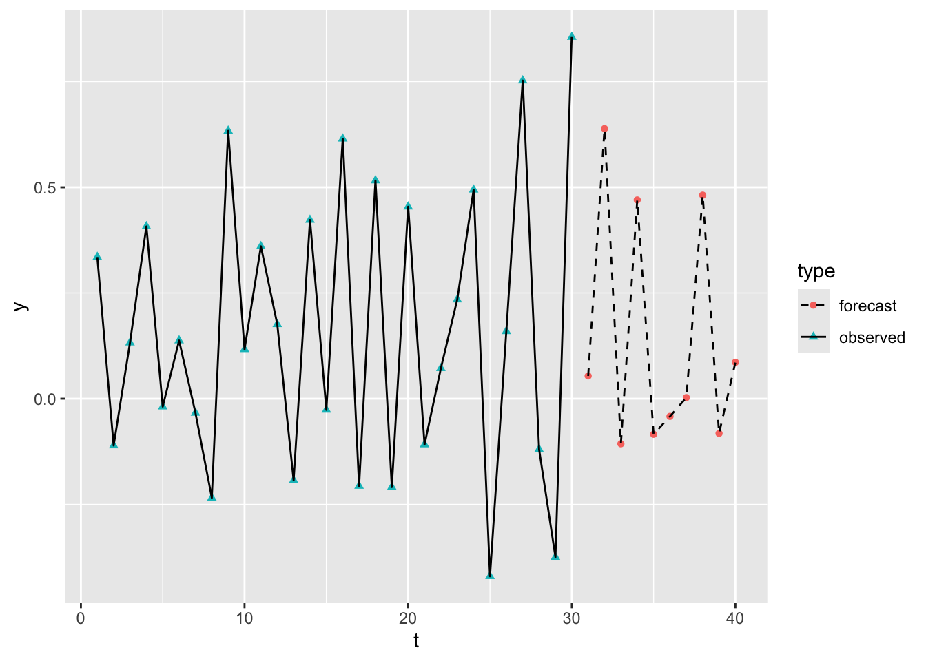
So we can see that the forecast sequence of values looks quite similar to the differenced observations before it.
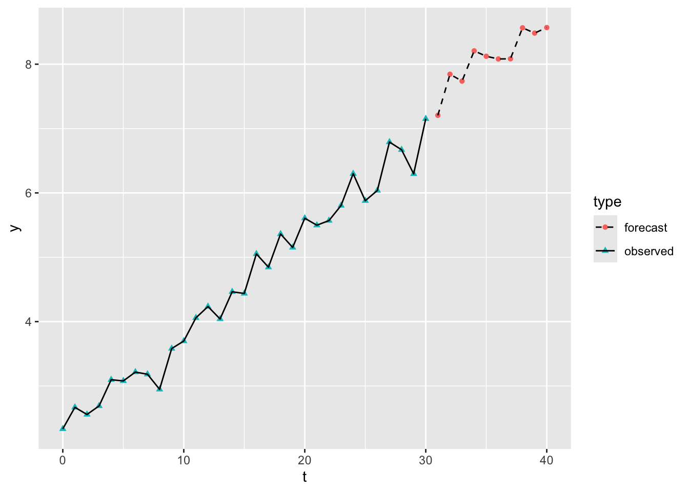
In order to use this for forecasting values, rather than differences, we therefore have to take the last observed value, and keep adding the consecutive forecast values.
So, after integrating (accumulating or summing up) the modelled differenced values, we now see the forecast values continuing the upwards trend observed in the original data.
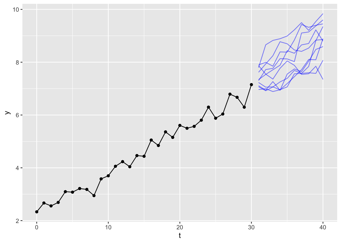
Of course, there’s nothing special about the specific sequence of draws generated from the model. We could run the same exercise multiple times and each time get a different sequence of model draws, and so a different forecast path. Let’s see ten draws, for example:
This gives a sense of the kinds of upwards-drifting walks are compatible with the amount of variation observed in the original data series. If we ran the experiment another 10 times, we would get another ten paths.
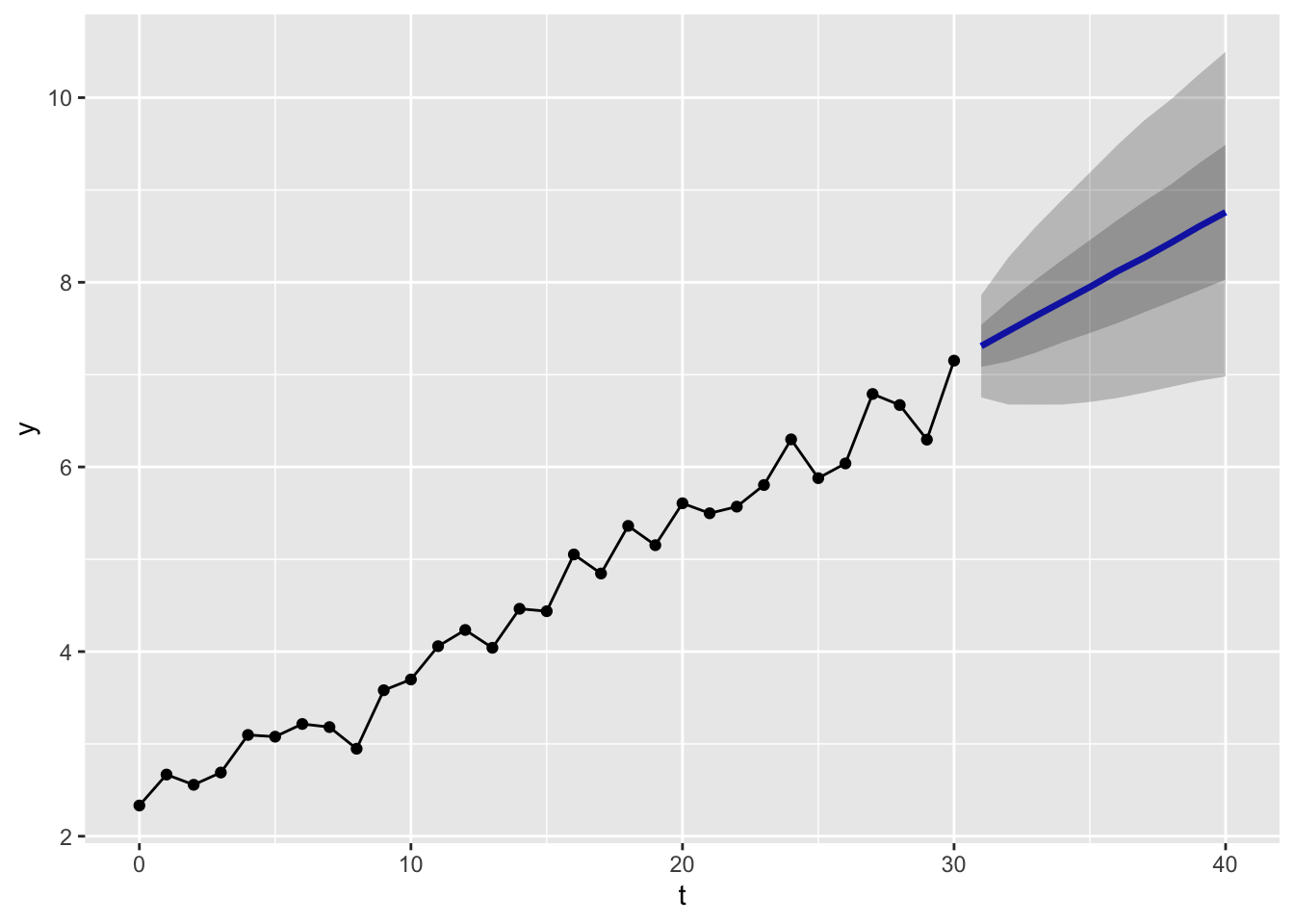
In fact, we could generate a much larger number of simulations, say 10,000, and then report the range of values within which (say) 50% or 90% of the values for each time period are contained:
These produce the kinds of ‘fans of uncertainty’ we might be used to seeing from a time series forecast. Because of the large numbers of simulations run, the shape of the fans appear quite smooth, and close to the likely analytical solution.
Summing up
In this post we’ve explored the second of the three main tools in the most common time series analytical toolkit: Integration. We’ve differenced our data once, which in time series parlance is represented by the shorthand d=1. Then we’ve integrated estimates we’ve produced from a model after differencing to represent random paths projecting forward from the observed data into a more uncertain future. Doing this multiple times has allowed us to represent uncertainty about these projections, and the ways that uncertainty increases the further we move from the observed data.
Coming up
In the next post, we will look at the final of the three tools in the standard time series toolkit: the moving average.
Footnotes
Hurray! We’ve demonstrated something we should know from school, namely that if \(y = \alpha + \beta x\), then \(\frac{\partial y}{\partial x} = \beta\).↩︎