Statistics as Circuit Boards

Introduction

The general approach I advocate for thinking about statistics is, for me, predicated on a series of related mental models for thinking about statistical inference and what we can do with statistical models. And these mental models are both graphical, and have some similarity with circuit board schematics, or more generally graphical representations of complex systems. To the extent these mental models have been useful for me, I hope they’ll be useful to others as well.

In the handwritten notes below I’ll try to show some of these mental models, and how they can help demystify some of the processes and opportunities involved in statistical inference

Terminology

Data for the model

As I recently discussed in a post relating to multivariate models, ultimately almost all models work with a big rectangle of data: each row an observation, each column a variable. We can call this big rectangle \(D\). Then, we need to imagine a way of splitting out this rectangle into two pieces: the model inputs (or predictor matrix), which we call \(X\), and the model outputs (or response matrix) which we call \(y\).

To try to represent this, I first thought about a big piece of square-lined paper, with a vertical perforation on it. Tear along this vertical perforation, and one of the pieces of paper is the output \(y\), and the other the input \(X\).

However, I then realised the \(X\)/\(y\) distinction is probably clearer to express symbolically as two complementary shapes: the input \(X\) being basically a rectangle with a right-facing chevron, and the output \(y\) being a rectangle with a chevron-shaped section missing from it on the left.

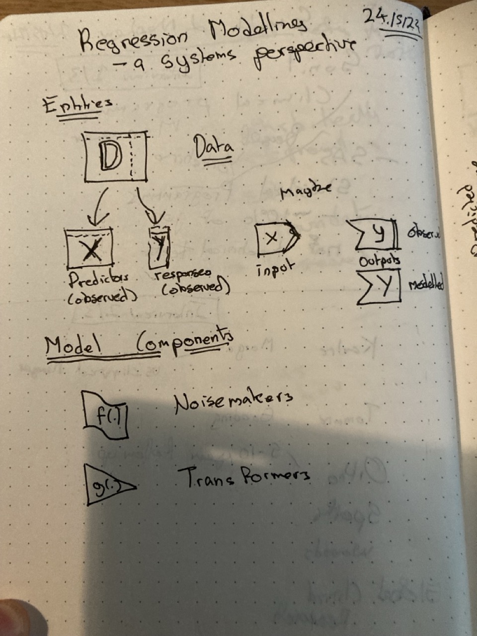
Model components

At a high enough level of generalisation, there are basically two component types that statistical models contain: stochastic components, denoted \(f(.)\), and deterministic components, denoted \(g(.)\). Within the figure, I’m referring to the deterministic components as transformers and the stochastic components as noisemakers. I decided to draw the transformers as triangles, and the noisemakers as ribbons.

Model fitting/calibration

Both transformers and noisemakers require specific parameters. Imagine these as a series of dials on two separate panels. The parameters for the transformers are usually referred to as \(\beta\) (‘beta’), which can be either (and rarely) a single value, or a vector of values. And the parameters for the noisemakers are usually referred to as \(\alpha\) (‘alpha’). There are many possible values of \(\beta\) and \(\alpha\) that a model can accept - many different ways the dials on the two panels can be set - and the main challenge of fitting a statistical model is to decide on the best configuration of \(\beta\) and \(\alpha\) to set the model to.

And what does ‘best’ mean? Broadly, that the discrepancy between what comes out of the model, \(Y\), and the corresponding outcome values in the dataset, \(y\), is minimised in some way. Essentially, this discrepancy, \(\delta\), is calculated with the current configuration of \(\beta\) and \(\alpha\), and then some kind of algorithm is applied to make a decision about how to adjust the dials. With the dials now adjusted, new model predictions \(Y\) are produced, leading to a new discrepancy value \(\delta\). If necessary, then the calibration algorithm is applied once again, so the \(\alpha\) and \(\beta\) parameters adjusted, and so the parameter operationalisation loop is repeated, until some kind of condition is met defining when the parameters identified are good enough.

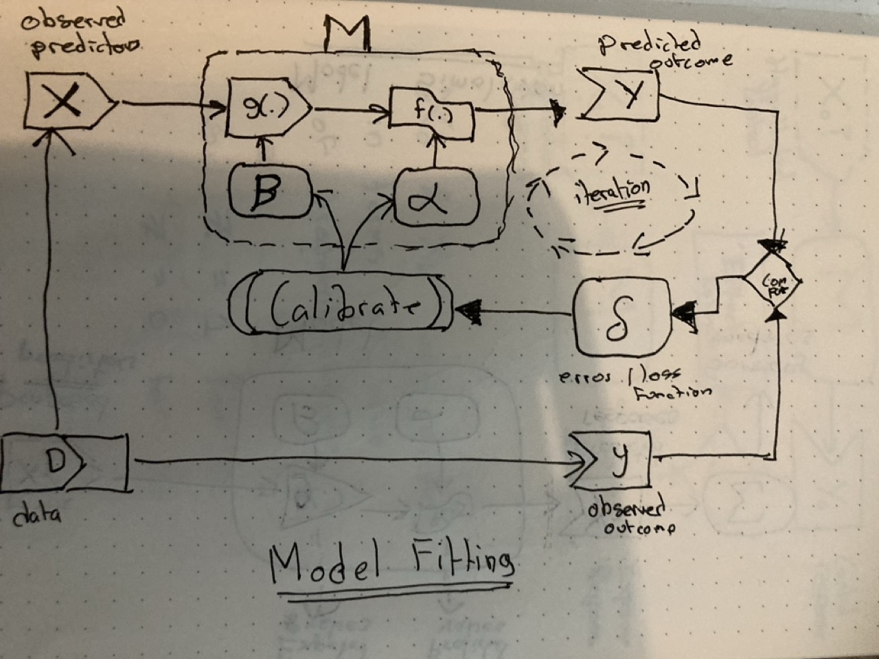
There are a number of possible ways of arriving at the ‘best’ parameter configuration. One approach is to employ an analytical solution, such as with the least-squares or generalised least-squares methods. In these cases some kind of algebraic ‘magic’ is performed and - poof! - the parameters just drop out instantly from the solution, meaning no repeated interation. In all other cases, however, it’s likely the predict-compare-calibrate cycle will be repeated many times, either until the error is deemed small enough, or until some kind of resource-based stopping condition - such as “stop after 10,000 tries” - has been reached.

This iterative cyclic quality of model fitting applies regardless of whether frequentist models - using maximum likelihood estimation - or Bayesian models - employing something like Hamiltonian Monte-Carlo estimation - have been employed. Both involve trying to minimise a loss function, i.e. the error \(\delta\) though updating the current best estimate of the parameter set \(\beta\) and \(\alpha\). ¹

Model simulation

Simple simulation

Once the model \(M\) has been calibrated, i.e. the best possible set of parameters \(\beta\) (for the transformer, \(g(.)\)) and \(\alpha\) (for the noisemaker, \(f(.)\)) have been identified in the calibration set, the model can now be used for prediction, projection, interpolation, extrapolation, and simulation more generally.

The challenges are two-fold: knowing how to ‘ask the model questions’; and knowing how to interpret the answers the model gives.

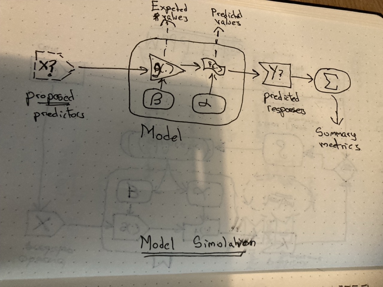
To ‘ask the model questions’, we need to specify some input data, \(X\), to put into the model. This input data could be taken from the same dataset used to calibrate the model in the first place. But it doesn’t have to be. We could ask the model to produce a prediction for configurations of input the model has never seen before. In this part of the complete example, we asked the model to predict levels of tooth growth where the dosage was between the dosage values in the dataset; this is an example of interpolation. In the same dataset we also saw examples of extrapolation, including dosage levels that were predicted/projected to lead to negative tooth growth, i.e. impossible values. So, a key challenge in asking questions of the model, through proposing an input predictor matrix \(X\), is to know which questions are and are not sensible to ask.

Knowing how to interpret the answers from the model is the second part of the challenge. If we run the model in its entirety, the values from the systematic component (transformer) are passed to the stochastic component (noisemaker), meaning we’ll get different answers each time.² For some types of model, we can just extract the results of the transformer part alone, and so produce expected values. If we pass the values from the transformer to the noisemaker, however, we’ll end up with a distribution of values from the model, even though the calibration parameters \(\beta\) and \(\alpha\), and input data \(X\) are non-varying. So, we may need to choose a way to summarise this distribution. For example, we may want to know the proportion of occasions/draws that exceed a particular threshold value \(\tau\). Or may want to calculate the median and a prediction interval.

Simulating ‘trials’

Once the fundamentals of simulation using statistical model simulations are understood, it’s just a small step to producing hypothetical simulation-based ‘trials’. Just apply two different input datasets \(X_0\) and \(X_1\) to the same model \(M\). These two datasets should differ only in terms of a specific exposure variable of interest \(Z\), with all other inputs kept the same. This is equivalent to magicking up the hypothetical ‘platinum standard’³ discussed in the course on causal inference: imagine exactly the same individual being observed in two different worlds, where only one thing (exposed/not exposed, or treated/not treated) is different.

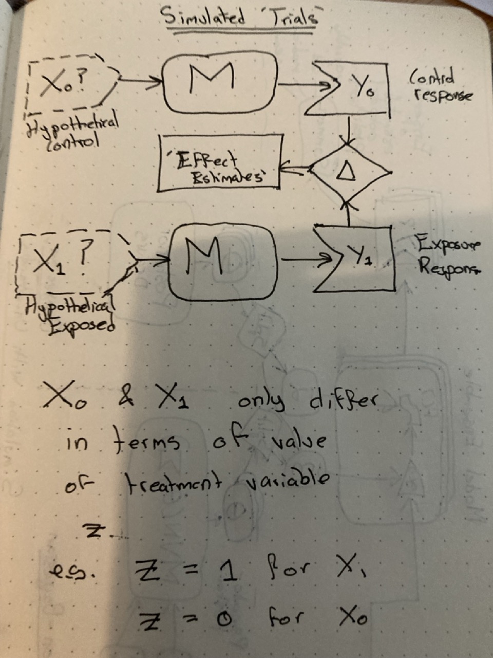
When it comes to intepretating the outputs, the job is now to compare between the outputs generated when \(X_0\) is passed to \(M\), and when \(X_1\) is passed to \(M\). Call these outputs \(Y_1\) and \(Y_0\) respectively; our treatment or exposure effect estimate is therefore the difference: \(Y_1 - Y_0\).

Simulating with honest uncertainty

Once you’re familiar with the last couple of steps - how to ‘ask models questions’, and how to ‘perform simulated trials’, the last challenge is how to do so honestly.

By honestly, I mean with appropriate acknowledgement of the effect that parameter uncertainty has on uncertainty in model outputs. We don’t really know the ‘true’ values of the parameter values \(\beta\) and \(\alpha\); we’ve just estimated them. And because they’re estimated, we’re not certain of their true value.

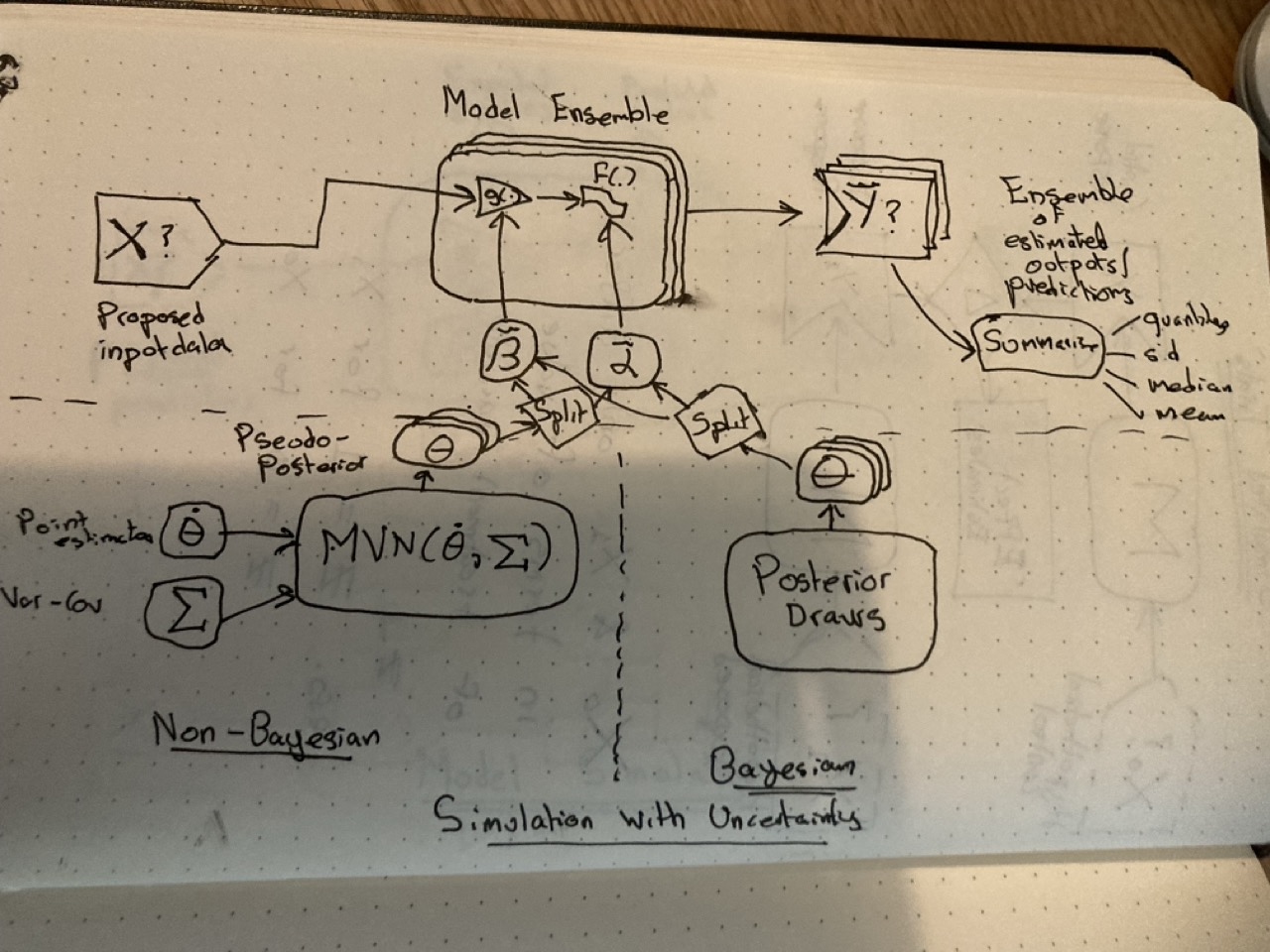
So, in order to represent the effect this parameter uncertainty has on the model outputs, there needs to be a way of generating and passing lots of ‘plausible parameter values’, \(\theta = \{ \beta, \alpha \}\), to the model. This means there’s a collection, or ensemble, of parameter values for the model, \(\tilde{\theta}\), and so an ensemble of models - each with a slightly different parameter configuration - that the predictor matrix \(X\) goes into.

And this then means that there’s an ensemble of model outputs, and so again a need to think about to summarise the distribution of outputs. Note that, because the variation in outputs comes about because of variation in the model parameters, a distribution of \(Y\) is generated even if the noisemakers (\(f(.)\)) are turned off, i.e. even if estimating for expected values rather than predicted values.

And how is the ensemble of parameter values produced? There are basically three approaches:

Analytical approximate solutions using something called the Delta Method: Not discussed here
Simulation methods involving normal approximations for frequentist-based models
Use the converged Bayesian posterior distribution.

In the figure, the Bayesian approach is shown on the right, and the simulation approach is shown on the left. A Bayesian converged posterior distribution is a distribution of plausible parameter values after the calibration process has been run enough times. It’s ideal for doing simulation with honest uncertainty, and was discussed back in the marbles-and-jumping-beans post. The downside is Bayesian models can take longer to run, and require more specialist software and algorithms to be installed/used.

The simulation approach for frequentist statistics was covered in the complete simulation example of the series, with its rationale developed over a few earlier posts. The basic aim of this approach is to generate an approximate analogue to the Bayesian posterior distribution, and this usually involves using a model to make inputs to feed into another model. It’s not quite models-all-the-way-down, but is a bit more meta than it may first appear!

Conclusion

This post aimed to re-introduce many of the key intuitions I’ve tried to develop in my main stats post series, but with a focus on the graphical intuition and concepts involved in statistical simulation, rather than just the algebra and R code examples. I hope this provides a useful complementary set of materials for thinking about statistical inference and statistical simulation. As mentioned at the start of the post, this is largely how I tend to think about statistical modelling, and so hopefully this way of thinking is useful for others who want to use statistical models more effectively too.

Footnotes

One crucial difference between the frequentist and Bayesian approaches is that, in the frequentist approach, a final set of parameter estimates is identified, equivalent to the dials on the panels being set a particular way and then never touched again. By contrast with the Bayesian approach the parameter set never quite stops changing, though it does tend to change less than it did at the start. The Bayesian approach is like a music producer who’s never quite satisfied with his desk, always tweaking this and that dial, though usually not by much. The technical definition is that frequentist parameter estimation converges to a point (hopefully), whereas Bayesian parameter estimation converges to a distribution (hopefully). This is what I was trying to express through the marble/jumping bean distinction here. The marble finds a position of rest; the jumping bean does not.↩︎
Though we can set a random number seed to make sure the different answers are the same each time.↩︎
If you’re a fan of the niche genre of sci-fi-rom-coms, you could also think of these as “sliding door moments”.↩︎