Part Twenty One: Time Series: The Moving Average Model
statistics
time series
Author
Jon Minton
Published
April 26, 2024
Recap
In the last couple of posts, we looked first at autoregression (the AR(p) model), then integration (represented by the term d), as part of a more general strategy for modelling time series data. In this post, we’ll complete the trilogy, by looking at the Moving Average (MA(q)) model.
The Moving Average Model in context of ARIMA
As with the post on autoregression, it’s worth returning to what I’ve been calling The Mother Model (a general way of thinking about statistical models), and how AR and I relate to it:
Stochastic Component
\[
Y_i \sim f(\theta_i, \alpha)
\]
Systematic Component
\[
\theta_i = g(X_i, \beta)
\]
To which we might also imagine adding a transformation or preprocessing step, \(h(.)\) on the dataset \(D\)
\[
Z = h(D)
\]
The process of differencing the data is the transformation step employed most commonly in time series modelling. This changes the types of values that go into both the data input slot of the mother model, \(X\), and the output slot of the mother model, \(Y\). The type of data transformer, however, is deterministic, hence the use of the \(=\) symbol. This means an inverse transform function, \(h^{-1}(.)\) can be applied to the transformed data to convert it back to the original data:
\[
D = h^{-1}(Z)
\]
The process of integrating the differences, including a series of forecast values from the time series models, constitutes this inverse transform function in the context of time series modelling, as we saw in the last post, on integration.
Autoregression is a technique for working with either the untransformed data, \(D\), or the transformed data \(Z\), which operates on the systematic component of the mother model. For example, an AR(3) autoregressive model, working on data which have been differenced once (\(Z_t = Y_t - Y_{t-1}\)), may look as follows:
Note that these two approaches, AR and I, have involved operating on the systematic component and the preprocessing step, respectively. This gives us a clue about how the Moving Average (MA) modelling strategy is fundamentally different. Whereas AR models work on the systematic component (\(g(.)\)), MA models work on the stochastic component (\(f(.)\)). The following table summarises the distinct roles each technique plays in the general time series modelling strategy:
AR, I, and MA in the context of ‘the Mother Model’
Technique
Works on…
ARIMA letter shorthand
Integration (I)
Data Preprocessing \(h(.)\)
d
Autoregression (AR)
Systematic Component \(g(.)\)
p
Moving Average (MA)
Stochastic Component \(f(.)\)
q
In the above, I’ve spoiled the ending! The Autoregressive (AR), Integration (I), and Moving Average (MA) strategies are commonly combined into a single model framework, called ARIMA. ARIMA is a framework for specifying a family of models, rather than a single model, which differ by the amount of differencing (d), or autoregression terms (p), or moving average terms (q) which the model contains.
Although in the table above, I’ve listed integration/differencing first, as it’s the data preprocessing step, the more conventional way of specifying an ARIMA model is in the order indicated in the acronym:
AR: p
I: d
MA: q
This means ARIMA models are usually specified with a three value shorthand ARIMA(p, d, q). For example:
ARIMA(1, 1, 0): AR(1) with I(1) and MA(0)
ARIMA(0, 2, 2): AR(0) with I(2) and MA(2)
ARIMA(1, 1, 1): AR(1) with I(1) and MA(1)
Each of these models is fundamentally different. But each is a type of ARIMA model.
With this broader context, about how MA models fit into the broader ARIMA framework, let’s now look at the Moving Average model:
The sound of a Moving Average
The intuition of a MA(q) model is in some ways easier to develop by starting not with the model equations, but with the following image:
Tibetan Singing Bowl
This is a Tibetan Singing Bowl, available from all good stockists (and Amazon), whose product description includes:
Ergonomic Design: The 3 inch singing bowl comes with a wooden striker and hand-sewn cushion which flawlessly fits in your hand. The portability of this bowl makes it possible to carry it everywhere you go.
Holistic Healing : Our singing bowls inherently produces a deep tone with rich quality. The resonance emanated from the bowl revitalizes and rejuvenates all the body, mind and spirit. It acts as a holistic healing tool for overall well-being.
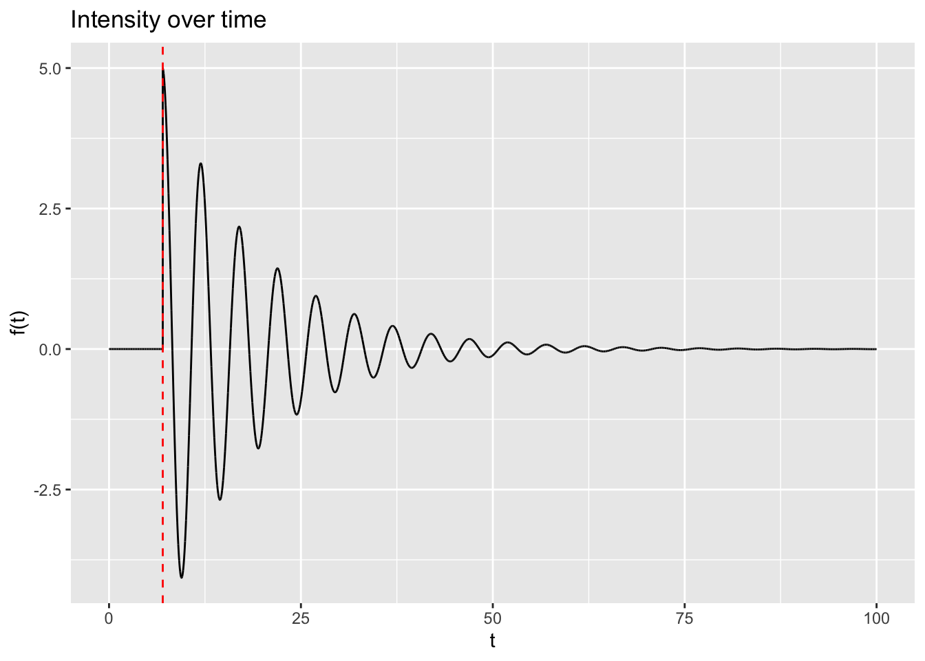
Notwithstanding the claims about health benefits and ergonomics, the bowl is something meant to be hit by a wooden striker, and once hit makes a sound. This sound sustains over time (‘sings’), but as time goes on the intensity decays. As a sound wave, this might look something like the following:
In this figure, the red dashed line indicates when the wooden striker strikes the bowl. Before this time, the bowl makes no sound. Directly after the strike, the bowl is loudest, and over time the intensity of the sound waves emanating from the bowl decays. The striker can to some extent determine the maximum amplitude of the bowl, whereas it’s largely likely to be the properties of the bowl itself which determines how quickly or slowly the sound decays over time.
How does this relate to the Moving Average model? Well, if we look at the Interpretation section of the moving average model wikipedia page, we see the cryptic statement “The moving-average model is essentially a finite impulse response filter applied to white noise”. And if we then delve into the finite impulse response page we get the definition “a finite impulse response (FIR) filter is a filter whose impulse response (or response to any finite length input) is of finite duration, because it settles to zero in finite time”. Finally, if we go one level deeper into the wikirabbit hole, and enter the impulse response page, we get the following definition:
[The] impulse response, or impulse response function (IRF), of a dynamic system is its output when presented with a brief input signal, called an impulse.
In the singing bowl example, the striker is the impulse, and the ‘singing’ of the bowl is its response.
The moving average equation
Now, finally, let’s look at the general equation for a moving average model:
Here is something like the fundamental value or quality of the time series system. For the singing bowl, \(\mu = 0\), but it can take any value. \(\epsilon_t\) is intended to capture something like a ‘shock’ or impulse now which would cause its manifested value to differ from its fundamental, \(\epsilon_{t-1}\) a ‘shock’ or impulse one time unit ago, and \(\epsilon_{t-2}\) a ‘shock’ or impulse two time units ago.
The values \(\theta_i\) are similar to the way the intensity of the singing bowl’s sound decays over time. They are intended to represent how much influence past ‘shocks’, from various recent points in history, have on the present value manifested. Larger values of \(\theta\) indicate past ‘shocks’ that have larger influence on the present value, and smaller \(\theta\) values less influence.
Autoregression and moving average: the long and the short of it
Autoregressive and moving average models are intended to be complementary in their function in describing a time series system: whereas Autoregressive models allow for long term influence of history, which can change the fundamentals of the system, Moving Average models are intended to represent transient, short term disturbances to the system. For an AR model, the system evolves in response to its past states, and so to itself. For a MA model, the system, fundamentally, never changes. It’s just constantly being ‘shocked’ by external events.
Concluding remarks
So, that’s the basic intuition and idea of the Moving Average model. A system fundamentally never changes, but external things keep ‘happening’ to it, meaning it’s almost always different to its true, fundamental value. A boat at sea will fundamentally have a height of sea level. But locally sea level is always changing, waves from every direction, and various intensities, buffetting the boat up and down - above and below the fundamental sea level average at every moment.
And the ‘sound’ of a moving average model is almost invariably likely to be less sonorous than that of a singing bowl. Instead of a neat sine wave, each shock is a random draw from a noisemaker (typically the Normal distribution). In this sense a more accurate analogy might not be a singing bowl, but a guitar amplifier, with a constant hum, but also with dodgy connections, constantly getting moved and adjusted, with each adjustment causing a short belt of white noise to be emanated from the speaker. A moving average model is noise layered upon noise.