One mapping line, two opposite conclusions

A worked example of the gg-spec round trip · Palmer penguins, TidyTuesday 2020-07-28

Published

August 18, 2026

Not a session page — a demonstration

This page shows the working method the sessions use: a plot is specified as a short YAML document of grammar-of-graphics mapping rules, the spec is compiled to ggplot2 code, the figure is rendered and looked at, and what looking reveals drives the next revision of the spec. How these sessions work.

In a live session, nobody types ggplot2 code to begin with. The group dictates mapping rules — which variable goes to which aesthetic, which geoms draw them, which scales transform them — and those rules are written down as a spec. The spec is short enough to argue about on a shared screen, and it is the record of the design decisions that ends up quoted in the writeup.

Here is one full round trip on the Palmer penguins data.

Reproducing this page

Runs from data/penguins.csv, committed in this repository. To refresh from source:

download.file(
  "https://raw.githubusercontent.com/rfordatascience/tidytuesday/main/data/2020/2020-07-28/penguins.csv",
  "data/penguins.csv")

Packages: tidyverse. Source: Horst, Hill & Gorman, palmerpenguins, via TidyTuesday 2020-07-28.

Code

library(tidyverse)
theme_set(theme_minimal(base_size = 13))

penguins <- read_csv("data/penguins.csv", show_col_types = FALSE) |>
  filter(!is.na(bill_depth_mm))

slope_pooled <- coef(lm(bill_depth_mm ~ bill_length_mm, data = penguins))[2]
slopes_species <- penguins |>
  group_by(species) |>
  group_modify(~ tibble(slope = coef(lm(bill_depth_mm ~ bill_length_mm, data = .x))[2])) |>
  ungroup()

Round 1: the spec as first dictated

The group asks a simple question — do penguins with longer bills also have deeper bills? — and dictates the minimal spec: two positional mappings, points, and a linear trend.

# Worked example, round 1 — compiled in example-gg-spec.qmd
data: penguins
filter: "!is.na(bill_depth_mm)"
mapping:
  x: bill_length_mm
  y: bill_depth_mm
layers:
  - geom: point
    alpha: 0.6
  - geom: smooth
    stat: lm
    se: true
labs:
  title: "Do longer bills mean deeper bills?"
  subtitle: "342 penguins, Palmer Archipelago 2007-09"
  x: "Bill length (mm)"
  y: "Bill depth (mm)"
theme: minimal

The spec compiles to code a reader could have written by hand — layers in spec order, nothing the spec didn’t ask for:

Code

ggplot(penguins, aes(x = bill_length_mm, y = bill_depth_mm)) +
  geom_point(alpha = 0.6) +
  geom_smooth(method = "lm", se = TRUE) +
  labs(
    title    = "Do longer bills mean deeper bills?",
    subtitle = sprintf("%d penguins, Palmer Archipelago 2007-09", nrow(penguins)),
    x = "Bill length (mm)", y = "Bill depth (mm)"
  )

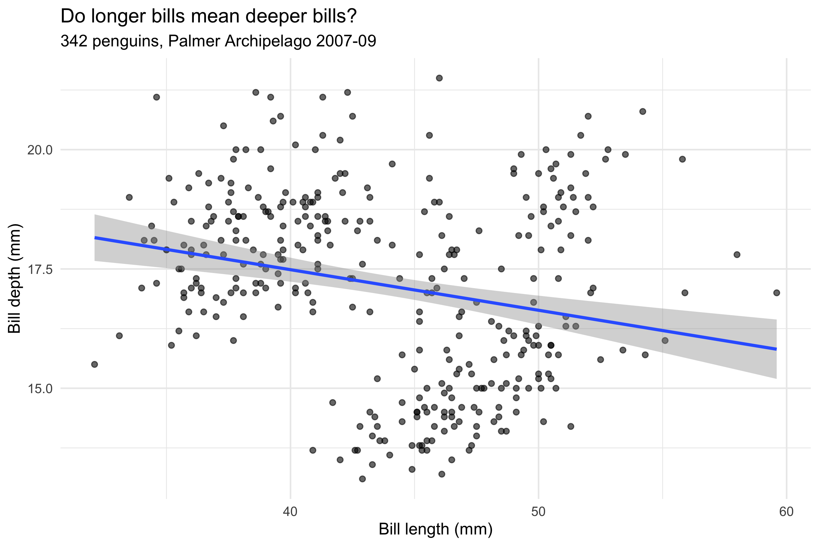
Figure 1: Round 1: bill depth against bill length, all penguins pooled. The fitted line slopes down.

Looking at the render

The fitted line says no: pooled across all 342 birds, each extra millimetre of bill length goes with 0.085 mm less depth. That contradicts any intuition about bigger birds having bigger bills — and looking at the point cloud shows why the line is suspect: the points sit in distinct clumps the spec has done nothing to distinguish.

The group’s diagnosis, in grammar terms: a variable that structures the data has been left out of the mapping. The fix is one line.

Round 2: one mapping line added

# Worked example, round 2 — one mapping line added: colour: species
data: penguins
filter: "!is.na(bill_depth_mm)"
mapping:
  x: bill_length_mm
  y: bill_depth_mm
  colour: species
layers:
  - geom: point
    alpha: 0.6
  - geom: smooth
    stat: lm
    se: true
scales:
  colour: okabe-ito
labs:
  title: "Within every species, the slope reverses"
  subtitle: "The same 342 penguins, now mapped by species"
  x: "Bill length (mm)"
  y: "Bill depth (mm)"
  colour: "Species"
theme: minimal

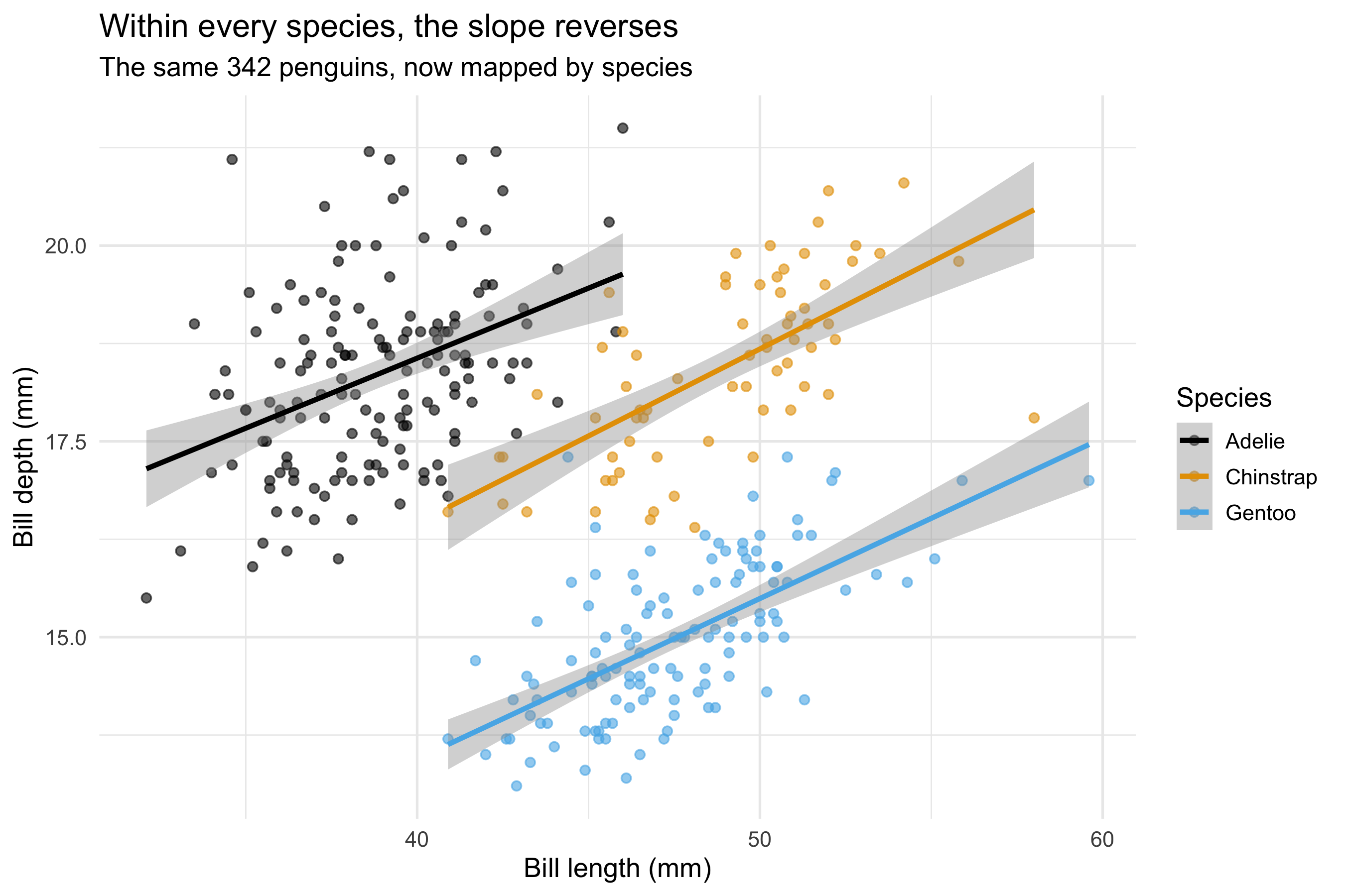
Only colour: species (and a colour-blind-safe scale for it) has been added. But because geom_smooth inherits the plot-level mapping, colour doesn’t just tint the points — it groups the stat, and one regression becomes three.

Code

ggplot(penguins, aes(x = bill_length_mm, y = bill_depth_mm, colour = species)) +
  geom_point(alpha = 0.6) +
  geom_smooth(method = "lm", se = TRUE) +
  scale_colour_manual(values = unname(palette.colors(3, palette = "Okabe-Ito"))) +
  labs(
    title    = "Within every species, the slope reverses",
    subtitle = sprintf("The same %d penguins, now mapped by species", nrow(penguins)),
    x = "Bill length (mm)", y = "Bill depth (mm)", colour = "Species"
  )

Figure 2: Round 2: the same data with species mapped to colour. Within every species the slope is positive.

Within each species the relationship runs the way intuition says it should — slopes of 0.18, 0.22, 0.20 mm per mm for Adelie, Chinstrap, Gentoo respectively, every one positive. The pooled negative slope was Simpson’s paradox: Gentoos are long-billed but shallow-billed, and pooling let the between-species contrast masquerade as a within-penguin trend.

What the round trip teaches

Mappings are decisions. The difference between the two figures — and two opposite conclusions — is a single line in the spec. Leaving a variable out of the mapping is as much a choice as putting it in.
Aesthetics reach further than appearance. Mapping colour regrouped the statistical layer, not just the ink. In the grammar, mappings feed stats, not only geoms.
The render is part of the method. The clumpy point cloud was visible in Round 1’s figure but nowhere in its spec or code. You find it by looking.

What the data can’t say

Three species from three islands over three seasons cannot separate species from island effects (Chinstraps and Gentoos were each sampled on effectively one island), and a within-species slope across individuals is still not a growth trajectory — no penguin was measured twice. The paradox here is a lesson about mappings, not a finding about penguins.

--- title: "One mapping line, two opposite conclusions" subtitle: "A worked example of the gg-spec round trip · Palmer penguins, TidyTuesday 2020-07-28" date: 2026-08-18 --- ::: {.callout-tip icon="false"} ## Not a session page — a demonstration This page shows the working method the sessions use: a plot is specified as a short YAML document of grammar-of-graphics mapping rules, the spec is compiled to ggplot2 code, the figure is rendered and *looked at*, and what looking reveals drives the next revision of the spec. [How these sessions work](index.qmd). ::: In a live session, nobody types ggplot2 code to begin with. The group dictates **mapping rules** — which variable goes to which aesthetic, which geoms draw them, which scales transform them — and those rules are written down as a spec. The spec is short enough to argue about on a shared screen, and it is the record of the design decisions that ends up quoted in the writeup. Here is one full round trip on the Palmer penguins data. ::: {.callout-tip collapse="true"} ## Reproducing this page Runs from `data/penguins.csv`, committed in this repository. To refresh from source: ``` r download.file( "https://raw.githubusercontent.com/rfordatascience/tidytuesday/main/data/2020/2020-07-28/penguins.csv", "data/penguins.csv") ``` Packages: `tidyverse`. Source: Horst, Hill & Gorman, [palmerpenguins](https://allisonhorst.github.io/palmerpenguins/), via TidyTuesday [2020-07-28](https://github.com/rfordatascience/tidytuesday/tree/main/data/2020/2020-07-28). ::: ```{r setup} library(tidyverse) theme_set(theme_minimal(base_size = 13)) penguins <- read_csv("data/penguins.csv", show_col_types = FALSE) |> filter(!is.na(bill_depth_mm)) slope_pooled <- coef(lm(bill_depth_mm ~ bill_length_mm, data = penguins))[2] slopes_species <- penguins |> group_by(species) |> group_modify(~ tibble(slope = coef(lm(bill_depth_mm ~ bill_length_mm, data = .x))[2])) |> ungroup() ``` ## Round 1: the spec as first dictated The group asks a simple question — do penguins with longer bills also have deeper bills? — and dictates the minimal spec: two positional mappings, points, and a linear trend. ```{r spec-1, echo=FALSE, results='asis'} cat("```yaml\n", paste(readLines("specs/penguins-example.yml"), collapse = "\n"), "\n```", sep = "") ``` The spec compiles to code a reader could have written by hand — layers in spec order, nothing the spec didn't ask for: ```{r fig-round-1} #| fig-cap: "Round 1: bill depth against bill length, all penguins pooled. The fitted line slopes down." ggplot(penguins, aes(x = bill_length_mm, y = bill_depth_mm)) + geom_point(alpha = 0.6) + geom_smooth(method = "lm", se = TRUE) + labs( title = "Do longer bills mean deeper bills?", subtitle = sprintf("%d penguins, Palmer Archipelago 2007-09", nrow(penguins)), x = "Bill length (mm)", y = "Bill depth (mm)" ) ``` ## Looking at the render The fitted line says *no*: pooled across all `r nrow(penguins)` birds, each extra millimetre of bill length goes with `r sprintf("%.3f", abs(slope_pooled))` mm *less* depth. That contradicts any intuition about bigger birds having bigger bills — and looking at the point cloud shows why the line is suspect: the points sit in distinct clumps the spec has done nothing to distinguish. The group's diagnosis, in grammar terms: **a variable that structures the data has been left out of the mapping**. The fix is one line. ## Round 2: one mapping line added ```{r spec-2, echo=FALSE, results='asis'} cat("```yaml\n", paste(readLines("specs/penguins-example-2.yml"), collapse = "\n"), "\n```", sep = "") ``` Only `colour: species` (and a colour-blind-safe scale for it) has been added. But because `geom_smooth` inherits the plot-level mapping, colour doesn't just tint the points — it **groups the stat**, and one regression becomes three. ```{r fig-round-2} #| fig-cap: "Round 2: the same data with species mapped to colour. Within every species the slope is positive." ggplot(penguins, aes(x = bill_length_mm, y = bill_depth_mm, colour = species)) + geom_point(alpha = 0.6) + geom_smooth(method = "lm", se = TRUE) + scale_colour_manual(values = unname(palette.colors(3, palette = "Okabe-Ito"))) + labs( title = "Within every species, the slope reverses", subtitle = sprintf("The same %d penguins, now mapped by species", nrow(penguins)), x = "Bill length (mm)", y = "Bill depth (mm)", colour = "Species" ) ``` Within each species the relationship runs the way intuition says it should — slopes of `r paste(sprintf("%.2f", slopes_species$slope), collapse = ", ")` mm per mm for `r paste(slopes_species$species, collapse = ", ")` respectively, every one positive. The pooled negative slope was Simpson's paradox: Gentoos are long-billed but shallow-billed, and pooling let the between-species contrast masquerade as a within-penguin trend. ## What the round trip teaches - **Mappings are decisions.** The difference between the two figures — and two opposite conclusions — is a single line in the spec. Leaving a variable out of the mapping is as much a choice as putting it in. - **Aesthetics reach further than appearance.** Mapping colour regrouped the statistical layer, not just the ink. In the grammar, mappings feed *stats*, not only geoms. - **The render is part of the method.** The clumpy point cloud was visible in Round 1's figure but nowhere in its spec or code. You find it by looking. ## What the data can't say Three species from three islands over three seasons cannot separate species from island effects (Chinstraps and Gentoos were each sampled on effectively one island), and a within-species slope across individuals is still not a growth trajectory — no penguin was measured twice. The paradox here is a lesson about mappings, not a finding about penguins.