---
title: "Global fertility: what's in the data"
subtitle: "Preparation · 2026-10-09 · Candidate grammar layer: geoms and stats"
date: 2026-10-09
---
```{r}
#| label: setup
#| include: false
library(tidyverse) # what other packages could be used?
gm <- read_csv(here::here("data/gapminder-fertility.csv"), show_col_types = FALSE)
pct_na <- function(x) scales::percent(mean(is.na(x)), accuracy = 0.1)
last_year <- function(v) max(gm$year[!is.na(gm[[v]])])
lowest <- slice_min(gm, fertility, n = 1, with_ties = FALSE)
highest <- slice_max(gm, fertility, n = 1, with_ties = FALSE)
```
::: {.callout-note icon="false"}
## Preparation notes, not a session writeup
These notes describe a candidate dataset before any session. The group has made no design decisions. The two Rosling-style figures were asked for by the facilitator as a familiar reference point, and the candidate mappings at the end are options for the group to choose from. Drafted by Claude Opus 5.5 from the output of `scripts/describe_data.R` and the Rdatasets documentation for `dslabs::gapminder`.
:::
The data is the `gapminder` table from Rafael Irizarry's [`dslabs`](https://cran.r-project.org/package=dslabs) package, which compiles [Gapminder](https://www.gapminder.org/data/) country indicators. It has one row per country per year, giving each country's total fertility rate (births per woman) alongside life expectancy, infant mortality, population and GDP.
::: {.callout-tip collapse="true"}
## Reproducing this page
The data is cached in `data/gapminder-fertility.csv`. To refresh it from the [Rdatasets copy](https://vincentarelbundock.github.io/Rdatasets/doc/dslabs/gapminder.html):
``` r
readr::read_csv("https://vincentarelbundock.github.io/Rdatasets/csv/dslabs/gapminder.csv") |>
  dplyr::select(-rownames) |>
  readr::write_csv("data/gapminder-fertility.csv")
```
Licence: `dslabs` is Artistic-2.0, and Gapminder's data is CC BY 4.0. Cite Gapminder.
:::
## The description
This is the verbatim output of the repository's deterministic describe script, so it is the same whichever agent runs it.
```{r}
#| label: describe
#| code-fold: false
#| comment: ""
rscript <- file.path(R.home("bin"), "Rscript")
cat(system2(rscript, c("--vanilla", here::here("scripts/describe_data.R"),
                       here::here("data/gapminder-fertility.csv")),
            stdout = TRUE), sep = "\n")
```
## Reading it
- **What it is.** Country indicators compiled by Gapminder, covering `r n_distinct(gm$country)` countries from `r min(gm$year)` to `r max(gm$year)`.
- **Grain.** One row per country per year, `r format(nrow(gm), big.mark = ",")` rows. There's no reshaping to do: the data is already tidy.
- **Types in grammar terms.** `fertility`, `life_expectancy`, `infant_mortality`, `population` and `gdp` are continuous. `year` is temporal and works as a continuous x. `continent` (`r n_distinct(gm$continent)` levels) is the only discrete variable in the range for colour or facets; `region` (`r n_distinct(gm$region)`) and `country` have too many levels for either.
- **Missingness has a shape.** `gdp` is `r pct_na(gm$gdp)` missing. It stops after `r last_year("gdp")` and is patchy before 1980. `fertility` (`r pct_na(gm$fertility)` missing) and `infant_mortality` (`r pct_na(gm$infant_mortality)`) have no values at all for `r max(gm$year)`, so in practice the fertility series ends in `r last_year("fertility")`. A line plot that runs to `r max(gm$year)` will stop short without warning.
- **Range.** Fertility runs from `r lowest$fertility` (`r lowest$country`, `r lowest$year`) to `r highest$fertility` (`r highest$country`, `r highest$year`).
## Rosling-style reference figures
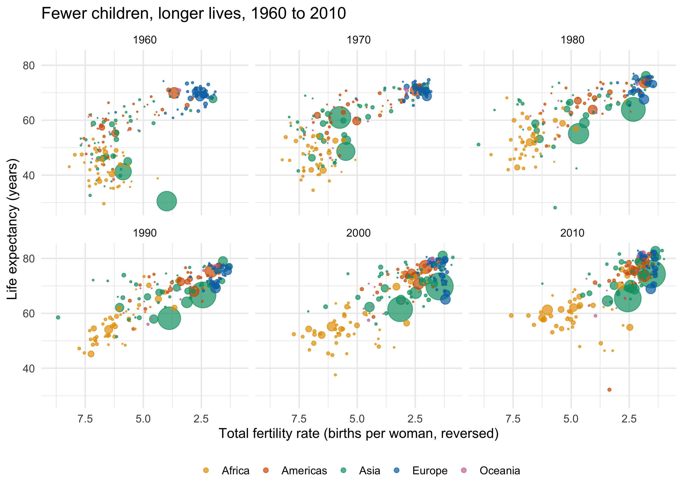
Anyone who watched Hans Rosling's talks will recognise these: fertility on x, life expectancy on y, one bubble per country sized by population and coloured by continent. They are here as a shared starting point to react to, not as the group's choices. The facilitator asked for them in preparation, and the group can keep, change or throw away any slot.
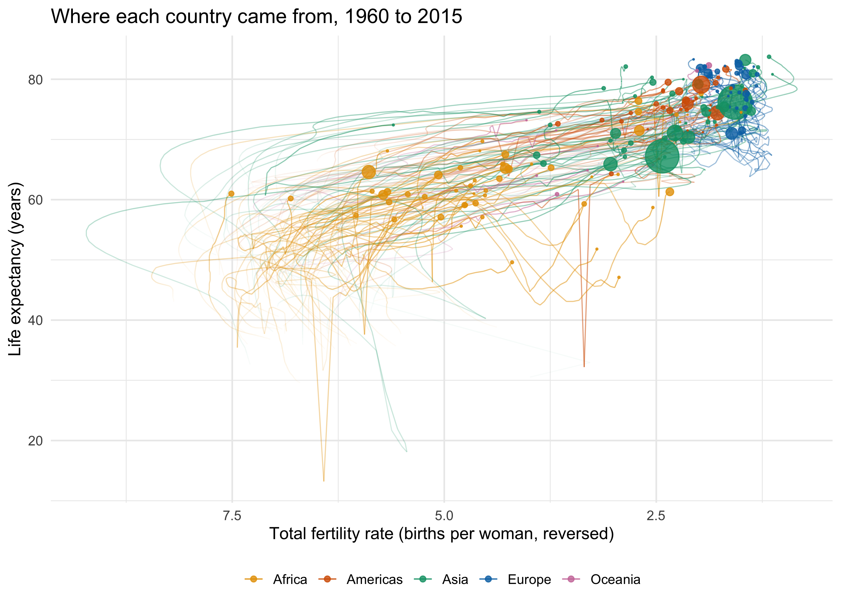
The animated original shows time by moving the bubbles. A static page has to put time somewhere else, and the two figures below make that choice in two different ways.
```{r}
#| label: rosling-data
decades <- seq(1960, 2010, by = 10)

rosling <- gm |>
  filter(!is.na(fertility), !is.na(life_expectancy), !is.na(population))

continent_cols <- c(Africa = "#E69F00", Americas = "#D55E00", Asia = "#009E73",
                    Europe = "#0072B2", Oceania = "#CC79A7") # Okabe-Ito
```
### Time as facets: one panel per decade
```{r}
#| label: fig-rosling-facets
#| fig-cap: "Each panel is one year at the start of a decade. Read across the panels to see the cloud of countries move from top left to bottom right."
#| fig-width: 9
#| fig-height: 6.5
rosling |>
  filter(year %in% decades) |>
  arrange(desc(population)) |> # draw big bubbles first so small ones stay visible
  ggplot(aes(x = fertility, y = life_expectancy,
             size = population, colour = continent)) +
  geom_point(alpha = 0.7) +
  facet_wrap(~ year) +
  scale_size_area(max_size = 12, guide = "none") +
  scale_colour_manual(values = continent_cols) +
  scale_x_reverse() +
  labs(x = "Total fertility rate (births per woman, reversed)",
       y = "Life expectancy (years)", colour = NULL,
       title = "Fewer children, longer lives, 1960 to 2010") +
  theme_minimal(base_size = 13) +
  theme(legend.position = "bottom")
```
The x axis is **reversed**, which is a decision to argue about. Reversed, the movement over time runs left to right, and "fewer births" sits on the same side as "longer lives". Rosling himself plotted fertility the natural way round (high on the right), so the countries moved right to left. Neither is wrong. But the choice changes what readers see as progress.
Two figures from the data anchor the panels. In `r min(decades)` the median country had `r median(rosling$fertility[rosling$year == min(decades)])` births per woman and a life expectancy of `r round(median(rosling$life_expectancy[rosling$year == min(decades)]), 1)`; by `r max(decades)` those medians were `r median(rosling$fertility[rosling$year == max(decades)])` and `r round(median(rosling$life_expectancy[rosling$year == max(decades)]), 1)`.
### Time as fading: older years more transparent
```{r}
#| label: fig-rosling-trails
#| fig-cap: "Each country's path from 1960 to 2015, fading into the past. The solid bubbles are the latest year with fertility data."
#| fig-width: 9
#| fig-height: 6.5
latest <- rosling |> filter(year == max(year))

rosling |>
  arrange(country, year) |>
  ggplot(aes(x = fertility, y = life_expectancy, colour = continent)) +
  geom_path(aes(group = country, alpha = year), linewidth = 0.4) +
  geom_point(data = latest, aes(size = population), alpha = 0.8) +
  scale_alpha_continuous(range = c(0.03, 0.6), guide = "none") +
  scale_size_area(max_size = 12, guide = "none") +
  scale_colour_manual(values = continent_cols) +
  scale_x_reverse() +
  labs(x = "Total fertility rate (births per woman, reversed)",
       y = "Life expectancy (years)", colour = NULL,
       title = paste0("Where each country came from, ", min(rosling$year),
                      " to ", max(rosling$year))) +
  theme_minimal(base_size = 13) +
  theme(legend.position = "bottom")
```
This version uses **alpha for time**, so older data is more faded. It keeps the movement in one panel, but the paths overlap heavily, and the faint tails are hard to read for any single country. Note the two layers here: the trails use all `r format(nrow(rosling), big.mark = ",")` rows, and the bubbles use a second data frame of only the latest year. That every layer can take its own `data` is itself a grammar point. It comes back on [the cross-silo page](nhs-cross-silo.qmd).
Looking at the rendered figures shows things the code doesn't. The few sudden vertical drops in life expectancy are not data errors. They are catastrophes: the large Asian bubble low in the 1960 panel is China (life expectancy `r gm$life_expectancy[gm$country == "China" & gm$year == 1960]`) during the famine that followed the Great Leap Forward, and the lone Americas point low in the 2010 panel is Haiti (`r gm$life_expectancy[gm$country == "Haiti" & gm$year == 2010]`) in the year of its earthquake. The trails show the same events as spikes.
Questions these two figures leave for the group:
- **Facets or alpha?** Facets give clean snapshots but lose each country's identity across panels. Alpha keeps identity and loses legibility.
- **Size.** Bubble area tracks population, so China and India dominate every panel. Is that the right emphasis for a question about *typical* countries?
- **The stat.** Both figures show raw points. A per-continent median path (a `stat_summary` layer) would be the geoms-and-stats lesson in one line of code.
## What the data can't say
These are national averages, so variation within a country is invisible, and every country counts equally whatever its population. The 1960s values for many countries are Gapminder's estimates and interpolations, not registered births. The record also ends before the recent falls in fertility.
## Candidate mappings (the group chooses)
``` text
Candidates (the group chooses) - gapminder-fertility:
  position x/y (continuous): fertility, life_expectancy, infant_mortality (14% NA),
                             population, gdp (28% NA, ends 2011)
  time:                      year (continuous, 1960-2015 usable for fertility)
  colour / facet (5 levels): continent
  size:                      population (spans 5 orders of magnitude)
  not for colour:            region (22), country (185) - filter or highlight a few
```
Why the data could suit **geoms and stats**: if you map year to x and fertility to y, you get `r format(sum(!is.na(gm$fertility)), big.mark = ",")` points, and those points can be drawn as dots, as one line per country, as a smoother per continent, or as a boxplot per decade. Choosing between those drawings is that session's lesson.