---
title: "Rolling Stone's greatest albums: the workbook"
subtitle: "Session 2 · TidyTuesday 2024-05-07 · Music sales and styles"
date: 2026-10-16
---
::: {.callout-tip icon="false"}
## Session 2 · 2026-10-16 · facilitated by Jon Minton
No one is named, because no consent record was taken. The room chose the dataset. This page is the session workbook, prepared by Claude Opus 5.5 from the session folder: `shortlist.md`, `notes.md`, and the specs and figures under `specs/` and `figures/`. It starts with the preparation and records each figure in the order it was made. The page was approved before publishing. [How these sessions work](../../index.qmd).
:::
::: {.callout-warning icon="false"}
## Where this workbook stands
The room chose the dataset. The spec trail records no graphic design decisions by the room: **spec 01 was proposed by the agent before the session**, and figure 02 was requested by the facilitator. Later specs will be added below as new numbered sections, quoted verbatim, each with its figure and what looking at the render showed.
:::
The brief for this session was music sales and musical styles. TidyTuesday has no dedicated music-sales week, so the shortlist offered four weeks that measure success in other ways: chart positions, critics' ranks and Spotify popularity. The room chose **Rolling Stone's "500 Greatest Albums of All Time"**: the 2003, 2012 and 2020 lists, merged into one table by The Pudding.
::: {.callout-tip collapse="true"}
## Reproducing this page
Runs from one CSV cached in `data/`. To refresh from source:
``` r
download.file(
  "https://raw.githubusercontent.com/rfordatascience/tidytuesday/main/data/2024/2024-05-07/rolling_stone.csv",
  "data/tt-2024-05-07-rolling_stone.csv")
```
Or use the repo's helper, which caches every file in the week: `sh scripts/workshop r scripts/tt_fetch.R 2024-05-07`.
Packages: `tidyverse`. Source: The Pudding, [*What makes an album the greatest of all time?*](https://pudding.cool/2024/03/greatest-music/), from Chris Eckert's spreadsheet, via TidyTuesday [2024-05-07](https://github.com/rfordatascience/tidytuesday/tree/main/data/2024/2024-05-07). No licence stated.
:::
```{r setup}
library(tidyverse)

rs <- read_csv("../../data/tt-2024-05-07-rolling_stone.csv", show_col_types = FALSE)

on_list <- rs |>
  transmute(`2003` = !is.na(rank_2003), `2012` = !is.na(rank_2012), `2020` = !is.na(rank_2020))
n_all_three <- sum(on_list$`2003` & on_list$`2012` & on_list$`2020`)
n_only_2020 <- sum(!on_list$`2003` & !on_list$`2012` & on_list$`2020`)
n_only_2003 <- sum(on_list$`2003` & !on_list$`2012` & !on_list$`2020`)

rs_2020 <- rs |> filter(!is.na(rank_2020))
```
## Step 1: choosing a dataset
The shortlist (`shortlist.md`) was scouted on the day of the session. Each week is listed with the grammar layer it stresses most. The series arc puts *geoms and stats* next, but which layer to cover was left for the room to decide. The room chose Rolling Stone, which stresses *scales and position* most.
| Week | What it is | Layer it stresses best | What it can't say |
|---|---|---|---|
| [2025-08-26](https://github.com/rfordatascience/tidytuesday/tree/main/data/2025/2025-08-26) Billboard Hot 100 #1s | Every US #1 single, 1958–2025, hand-coded for genre, tempo and 54 instrument flags | Geoms and stats | Only the songs that reached #1; the codes are one listener's judgement |
| [2024-05-07](https://github.com/rfordatascience/tidytuesday/tree/main/data/2024/2024-05-07) Rolling Stone Album Rankings | 691 albums on the 2003, 2012 or 2020 "500 Greatest" lists | Scales and position | Critics' rankings, not sales; the voter panel changed between lists |
| [2020-09-29](https://github.com/rfordatascience/tidytuesday/tree/main/data/2020/2020-09-29) Beyoncé and Taylor Swift | Copies sold per album and country, plus national chart peaks | Scales | Two artists, patchy country coverage, worldwide rows that include the country rows |
| [2020-01-21](https://github.com/rfordatascience/tidytuesday/tree/main/data/2020/2020-01-21) Spotify Songs | About 28,000 tracks with audio features, in 6 genres | Facets and stats | Genre belongs to the playlist, not the track |
The only real sales figures are in the 48-row Beyoncé and Taylor Swift table. Every other week stands in for sales with a proxy.
## Step 2: describing the data
This step follows the tt-fetch skill's description of the week (the `notes.md` summary). The numbers here are recomputed from the cached CSV.
**Grain: one row per album.** The table has `r nrow(rs)` rows and `r ncol(rs)` columns. An album appears once, whichever lists it was on. A missing rank means "not on that list", so each rank column is about `r scales::percent(mean(is.na(rs$rank_2020)), 1)` missing. That missingness carries information; it is not lost data.
```{r overlap}
on_list |>
  count(`2003`, `2012`, `2020`, name = "albums") |>
  mutate(across(`2003`:`2020`, \(x) if_else(x, "✓", ""))) |>
  arrange(desc(albums))
```
`r n_all_three` albums are on all three lists. `r n_only_2020` appear only in 2020 and `r n_only_2003` only in 2003. One row is on none of the three lists.
| Variable | Type (grammar terms) | Notes |
|---|---|---|
| `rank_2003`, `rank_2012`, `rank_2020` | continuous, reversed | 1 is best, so the scale must be reversed. 2003 has `r sum(duplicated(na.omit(rs$rank_2003)))` tied ranks |
| `differential` | derived | 2003 rank minus 2020 rank, with a missing rank counted as 501. Recompute it before using it |
| `release_year` | continuous (or temporal) | `r min(rs$release_year)`–`r max(rs$release_year)` |
| `peak_billboard_position` | continuous, with a code | 201 means "never charted" (`r sum(rs$peak_billboard_position == 201, na.rm = TRUE)` albums), not a position |
| `weeks_on_billboard` | continuous, long right tail | up to `r max(rs$weeks_on_billboard, na.rm = TRUE)`; `r scales::percent(mean(is.na(rs$weeks_on_billboard)), 1)` missing |
| `spotify_popularity` | continuous | a snapshot from when the data was collected |
| `genre` | discrete (`r n_distinct(na.omit(rs$genre))` levels) | `r scales::percent(mean(is.na(rs$genre)), 1)` missing; "Blues/Blues ROck" is a misspelled duplicate |
| `type` | discrete (`r n_distinct(rs$type)` levels) | `r scales::percent(mean(rs$type == "Studio", na.rm = TRUE), 1)` Studio |
| `artist_gender` | discrete (`r n_distinct(na.omit(rs$artist_gender))` levels) | Male, Female, Male/Female |
| `artist_member_count` | discrete or continuous | whole numbers 1–12; how to treat it is the room's decision |
| `album`, `clean_name`, `album_id`, `spotify_url` | identifiers | labels only |
The agent **proposed** these candidate mappings. None of them is a choice:
- a slope or bump chart of rank across the three lists, which has to handle albums that join or leave a list
- release year against 2020 rank, coloured by genre or gender, to see which eras the 2020 voters rewarded
- critics against the market: peak Billboard position or weeks on the chart against rank, which needs decisions about the 201 code and a log axis
- small multiples by `type` or `genre`
## Step 3: spec 01, a starting point
::: {.callout-important icon="false"}
## Proposed by the agent, not decided by the room
The facilitator asked for a first figure to have on screen before the session. Claude Opus 5.5 filled every slot in this spec. The room has not chosen any of it, and it is there to be revised or thrown away.
:::
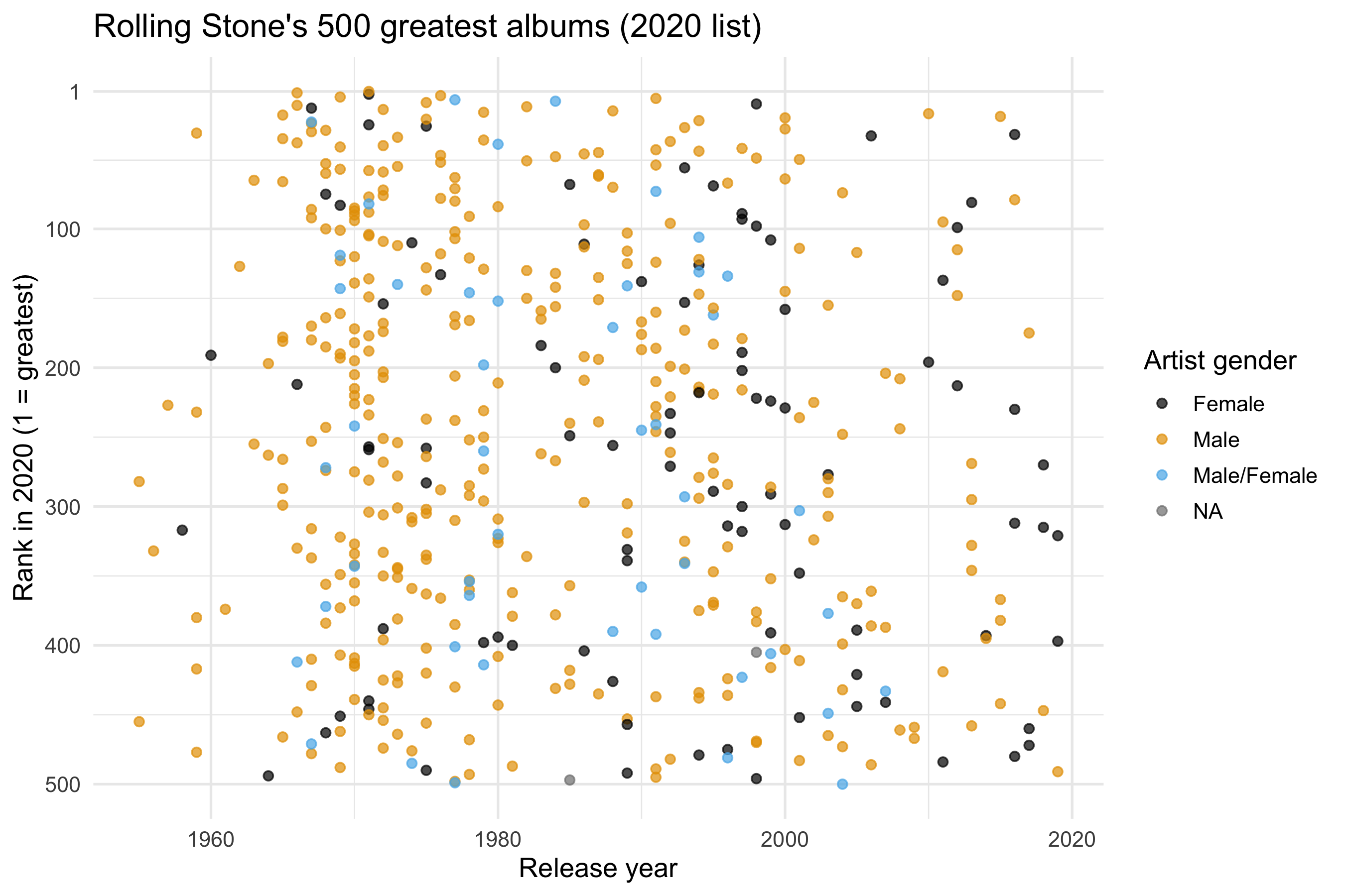
The question the agent chose was: *which release eras did the 2020 list reward, and where in the ranking?*
``` yaml
# sessions/2026-10-16/specs/01-rs-era-2020.yml
data: tt-2024-05-07-rolling_stone
filter: "!is.na(rank_2020)"   # grain: one row per album on the 2020 list
mapping:
  x: release_year
  y: rank_2020
  colour: artist_gender
layers:
  - geom: point
    alpha: 0.7
scales:
  y: scale_y_reverse(breaks = c(1, 100, 200, 300, 400, 500))
  colour: okabe-ito
labs:
  title: "Rolling Stone's 500 greatest albums (2020 list)"
  x: "Release year"
  y: "Rank in 2020 (1 = greatest)"
  colour: "Artist gender"
theme: minimal
```
```{r fig-spec-01}
#| fig-alt: "Scatter of the 500 albums on Rolling Stone's 2020 list: release year on x, rank on a reversed y axis with 1 at the top, points coloured by artist gender. Points are densest from the mid-1960s to the late 1970s and spread evenly from top to bottom."
ggplot(rs_2020, aes(x = release_year, y = rank_2020, colour = artist_gender)) +
  geom_point(alpha = 0.7) +
  scale_y_reverse(breaks = c(1, 100, 200, 300, 400, 500)) +
  scale_colour_manual(values = unname(palette.colors(3, palette = "Okabe-Ito"))) +
  labs(
    title = "Rolling Stone's 500 greatest albums (2020 list)",
    x = "Release year",
    y = "Rank in 2020 (1 = greatest)",
    colour = "Artist gender"
  ) +
  theme_minimal(base_size = 13)
```
Looking at the render:
- **The y axis carries no density.** Each rank from 1 to 500 is used once, so the points are spread evenly from top to bottom by construction. Everything the figure shows is in how release years spread *along* each band of ranks. The eye reads clusters left to right, not top to bottom.
- **The pattern is in the x distribution, and points are a weak way to show it.** The 1970s alone hold `r sum(between(rs_2020$release_year, 1970, 1979))` of the 500 albums, and at `alpha = 0.7` the points from 1965 to 1975 merge into a block. The correlation between release year and rank is only `r sprintf("%.2f", cor(rs_2020$release_year, rs_2020$rank_2020))`. If there is an era effect, this geom does not make it visible.
- **Colour shows counts, not shares.** `r sum(rs_2020$artist_gender == "Male", na.rm = TRUE)` of the 500 albums are by male artists, so the female and mixed points are scattered among them. Whether women's share rises in later decades is a proportion per decade, which is a stat the spec does not compute.
- **Two defaults nobody decided on.** Okabe-Ito's first colour is black, and levels are assigned alphabetically, so "Female" gets the heaviest ink by accident. The legend also has an `NA` entry: the `r sum(is.na(rs_2020$artist_gender))` albums on the 2020 list with no artist gender are both "Various Artists" compilations.
- The title fits at 9 inches, and the reversed axis with 1 at the top reads correctly.
All of these point at the **geoms and stats** layer: the same mapping could be drawn as something other than points. Some candidate first moves are listed below. They are proposals, at most three per slot, as in gg-spec's interactive mode.
| Slot | Options to put to the room |
|---|---|
| Geom/stat for the era question | histogram or density of `release_year`, faceted or filled by rank band (top 100 / 101–250 / 251–500); boxplot or `ggdist` interval of `release_year` per rank band; keep points and add a smoother |
| The gender question | bars of the proportion of each gender per release decade (`position = "fill"`); drop colour and answer the era question first; keep colour but put Male in grey |
| The `NA` gender rows | filter them out and say so in a caption; label them "Compilation"; leave them as they are |
<!--
LIVE SESSION ROUNDS — one section per spec, appended as the room dictates them.
For each: the decision in grammar terms (what was considered, what was chosen, why),
the YAML verbatim from specs/NN-*.yml, a chunk that compiles it with ../../data paths,
and "Looking at the render" bullets with inline r numbers. Forks get sibling numbers.
## Step 5: spec 03, <the room's next revision>
-->
## Step 4: figure 02, the genre of each list's top five
::: {.callout-important icon="false"}
## Requested by the facilitator, with one assumption by the agent
The facilitator asked for "the assumed genre of the top five over time, as something like a Sankey chart". Claude Opus 5.5 made the remaining choices: an alluvial layout, an "Outside top 5" block, the colours and the album labels. It also made the genre assumption described below. This figure is outside the gg-spec schema, because its geoms come from the [`ggalluvial`](https://corybrunson.github.io/ggalluvial/) extension rather than from ggplot2 itself. So it is recorded as a script (`specs/02-top5-genre-sankey.R`), not as YAML.
:::
```{r top5-data}
library(ggalluvial)

assumed_genre <- "Rock/Pop (assumed)"
outside       <- "Outside top 5"

top5_albums <- rs |>
  filter(pmin(rank_2003, rank_2012, rank_2020, na.rm = TRUE) <= 5)

top5 <- top5_albums |>
  mutate(
    genre = replace_na(genre, assumed_genre),
    album = recode(album, "Sgt. Pepper's Lonely Hearts Club Band" = "Sgt. Pepper's")
  ) |>
  pivot_longer(starts_with("rank_"), names_to = "list", names_prefix = "rank_",
               values_to = "rank") |>
  mutate(
    position = if_else(rank <= 5, genre, outside),
    position = fct_relevel(factor(position), outside, after = Inf),
    genre    = fct_relevel(factor(genre), assumed_genre)
  )

in_top5    <- \(yr) top5 |> filter(list == yr, rank <= 5)
n_assumed  <- sum(is.na(top5_albums$genre))
rock_2003  <- sum(in_top5("2003")$genre == assumed_genre)
rock_2020  <- sum(in_top5("2020")$genre == assumed_genre)
soul_2020  <- sum(in_top5("2020")$genre == "Soul/Gospel/R&B")
same_03_12 <- setequal(in_top5("2003")$album, in_top5("2012")$album)
rank_20    <- \(a) top5 |> filter(list == "2020", album == a) |> pull(rank)
```
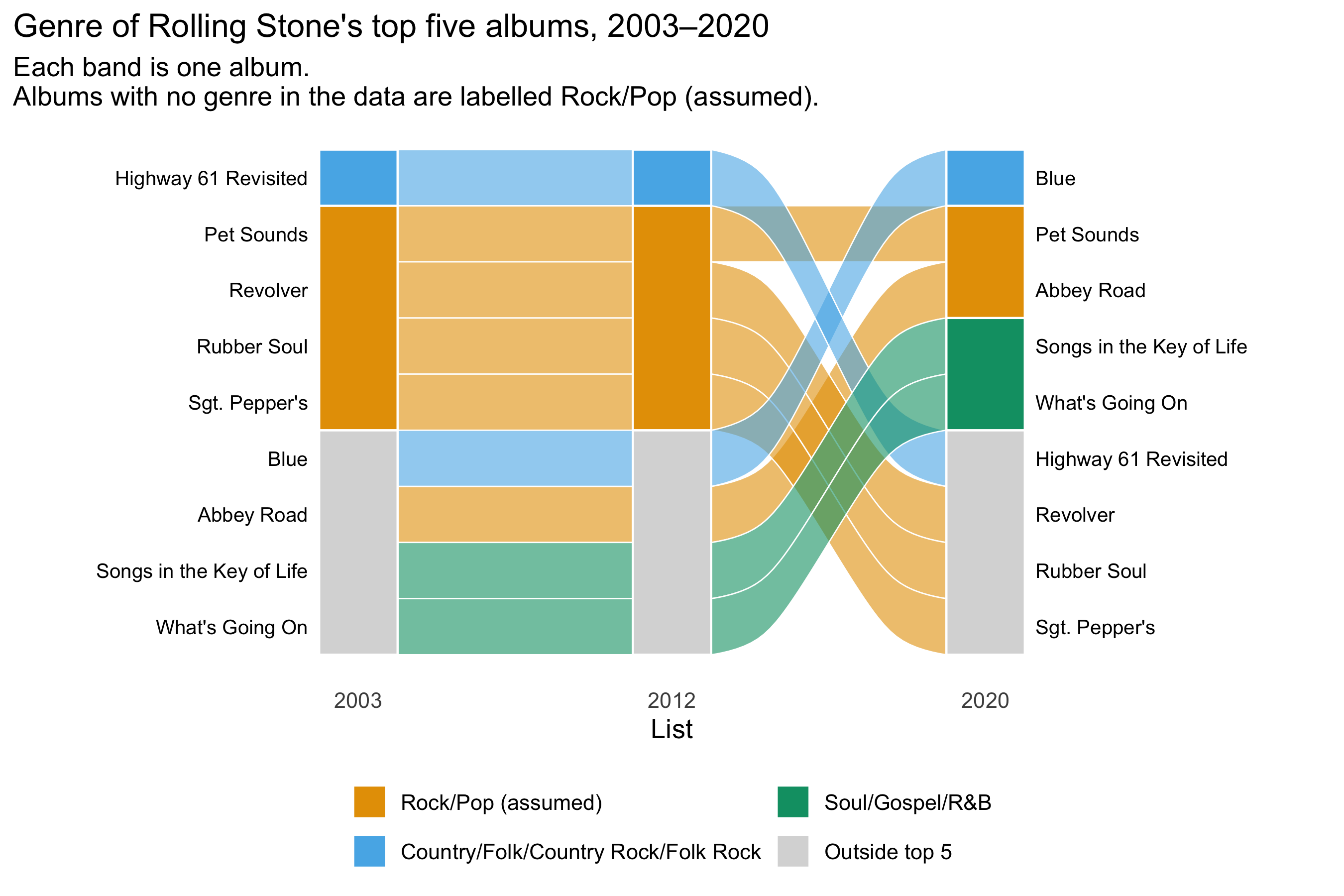
**The assumption.** `r nrow(top5_albums)` albums have been in at least one list's top five. `r n_assumed` of them have no genre in the data, and all of them are by the Beatles or the Beach Boys. None of the dataset's 16 genre groups is plain rock or pop, which suggests the coders left mainstream rock and pop blank. So these albums are labelled **Rock/Pop (assumed)**, and the label says it is an assumption. The data says nothing about why the genre is missing.
```{r fig-top5-sankey}
#| fig-alt: "Alluvial chart of the nine albums that were ever in a Rolling Stone top five, across the 2003, 2012 and 2020 lists. The 2003 and 2012 top fives are identical: four assumed Rock/Pop albums and Highway 61 Revisited. In 2020 Revolver, Rubber Soul, Sgt. Pepper's and Highway 61 Revisited flow out, and Blue, Abbey Road, Songs in the Key of Life and What's Going On flow in."
genre_cols <- c(
  set_names(unname(palette.colors(4, palette = "Okabe-Ito"))[2:4], levels(top5$genre)),
  set_names("grey85", outside)
)

ggplot(top5, aes(x = list, stratum = position, alluvium = album, y = 1, fill = genre)) +
  geom_alluvium(alpha = 0.6, width = 1/4, colour = "white", linewidth = 0.3) +
  geom_stratum(aes(fill = position), width = 1/4, colour = "white") +
  geom_text(stat = "alluvium", hjust = 1, nudge_x = -0.16, size = 3.4, na.rm = TRUE,
            aes(label = after_stat(if_else(x == 1, as.character(alluvium), NA)))) +
  geom_text(stat = "alluvium", hjust = 0, nudge_x = 0.16, size = 3.4, na.rm = TRUE,
            aes(label = after_stat(if_else(x == 3, as.character(alluvium), NA)))) +
  scale_x_discrete(expand = expansion(add = c(1.1, 1.1))) +
  scale_fill_manual(values = genre_cols, breaks = names(genre_cols)) +
  labs(
    title = "Genre of Rolling Stone's top five albums, 2003–2020",
    subtitle = "Each band is one album.\nAlbums with no genre in the data are labelled Rock/Pop (assumed).",
    x = "List", y = NULL, fill = NULL
  ) +
  theme_minimal(base_size = 13) +
  theme(axis.text.y = element_blank(), panel.grid = element_blank(),
        legend.position = "bottom") +
  guides(fill = guide_legend(nrow = 2))
```
Looking at the render:
- **Nothing moves between 2003 and 2012.** `r if (same_03_12) "The two lists have the same top five" else "The two top fives differ"`, so the left half of the chart is flat bands. All the change happens in 2020, the list with the new panel of voters.
- **In 2020 the assumed Rock/Pop albums fall from `r rock_2003` of the top five to `r rock_2020`, and Soul/Gospel/R&B goes from none to `r soul_2020`.** *Sgt. Pepper's* falls to `r rank_20("Sgt. Pepper's")`, *Revolver* to `r rank_20("Revolver")` and *Rubber Soul* to `r rank_20("Rubber Soul")`. *Abbey Road* rises into the top five. The Rock/Pop assumption decides how that shift looks: label those albums differently and the story changes.
- **"Outside top 5" is not "dropped off the list".** All `r nrow(top5_albums)` albums are on all three lists. The grey block hides how far each one fell or rose. A slope chart of rank would show it, and this layout cannot.
- **The first render had the labels on the wrong ribbons.** It used `geom_flow()` for the bands and `stat = "alluvium"` for the labels. The two stats sort albums differently inside a block, so in 2003 the "Blue" label sat on an orange ribbon. The code gave no warning; only looking at the render caught it. Drawing each album as one continuous `geom_alluvium()` puts the bands and labels in the same order.
- With only nine albums, every band is one album (`y = 1`). The chart is closer to a bump chart drawn as ribbons than to a Sankey of quantities.
## Decisions and pain points so far
- **No sales week exists.** The brief asked for sales, but only the 48-row Beyoncé and Taylor Swift table has sales figures. Every candidate uses a proxy, and the choice of proxy (critics, charts or streams) shapes the question before any mapping is made.
- **No licence is stated** for any shortlisted week. These weeks are fine as live teaching material, but derived data should not be republished on this page until the source has been checked.
- **Missing means "not on the list".** Treating a missing rank as zero, or dropping those rows silently, would change what any cross-list figure says. Spec 01 avoids the problem by filtering to the 2020 list, which also means it can't say anything about the albums that dropped off.
- **`differential` is derived and inconsistent** (a missing rank is counted as 501). Any figure about change between lists should recompute it.
## What the data can't say
These are critics' rankings, not sales or listening figures. For 2020 Rolling Stone polled a new panel of voters, so a change in an album's rank mixes changing taste with a change of voters. Even a clear rise in recent albums would not show that tastes had changed. The Billboard and Spotify columns are US-centric, and Spotify popularity is a single snapshot from when the data was collected. A "500 greatest" list is also censored at the top: it says nothing about the albums ranked 501st and below, and the `r n_only_2003` albums that appear only in 2003 simply drop out of a 2020-only figure.