---
title: "Two silos, one plot: A&E waits and delayed discharges"
subtitle: "Preparation · 2026-10-09 · Candidate grammar layer: data, and layers with their own data"
date: 2026-10-09
---
```{r}
#| label: setup
#| include: false
library(tidyverse)
library(patchwork)
ae_raw <- read_csv(here::here("data/phs-ae-monthly.csv"), show_col_types = FALSE)
dd_raw <- read_csv(here::here("data/phs-delayed-discharge.csv"), show_col_types = FALSE)
boards <- read_csv(here::here("data/phs-health-boards.csv"), show_col_types = FALSE) |>
filter(is.na(HBDateArchived)) |>
transmute(HBT = HB, board = str_remove(HBName, "^NHS "))
yyyymm <- function(x) ym(as.character(x)) # PHS codes months as 202608, not as dates
# Silo 1: emergency departments (Type 1 sites), all attendances, board x month
ed <- ae_raw |>
filter(DepartmentType == "Type 1", AttendanceCategory == "All") |>
group_by(HBT, month = yyyymm(Month)) |>
summarise(attendances = sum(NumberOfAttendancesAll),
within_4h = sum(NumberWithin4HoursAll), .groups = "drop") |>
mutate(pct_4h = within_4h / attendances) |>
left_join(boards, by = "HBT")
ed_scot <- ed |>
group_by(month) |>
summarise(attendances = sum(attendances), within_4h = sum(within_4h)) |>
mutate(pct_4h = within_4h / attendances)
# Silo 2: delayed discharges, adults, all delay reasons, board x month
delays <- dd_raw |>
filter(AgeGroup == "18plus", ReasonForDelay == "All Delay Reasons") |>
transmute(HBT, month = yyyymm(MonthOfDelay),
bed_days = NumberOfDelayedBedDays,
delayed_beds = AverageDailyNumberOfDelayedBeds)
delays_scot <- delays |> filter(HBT == "S92000003")
delays_hb <- delays |> filter(HBT != "S92000003") |> left_join(boards, by = "HBT")
# The cross-silo join: board and month are the shared keys
both_scot <- inner_join(ed_scot, delays_scot, by = "month")
both_hb <- inner_join(ed, delays_hb, by = c("HBT", "board", "month"))
first_m <- min(both_scot$month)
last_m <- max(both_scot$month)
fmt_m <- function(d) format(d, "%B %Y")
pct <- function(x) scales::percent(x, accuracy = 1)
at <- function(d, v) both_scot[[v]][both_scot$month == d]
r_scot <- cor(both_scot$delayed_beds, both_scot$pct_4h)
```
::: {.callout-note icon="false"}
## Preparation notes, not a session writeup
These notes propose a dataset and question for a possible session. Nothing here is a decision by a group. The figures are the agent's first drafts for a facilitator to react to, and are labelled as such. Drafted by Claude Opus 5.5 after a planning conversation about cross-silo analysis in NHS performance work, from Public Health Scotland open data.
:::
## Why this question
Health-service analysts tend to work one silo at a time. Emergency department waiting times are published and analysed by one team, and delayed discharges by another. Ambulance handovers belong to a third. Each team's output is a chart of its own measure.
But patient flow doesn't respect those boundaries. A patient who is medically fit to leave hospital but can't, because no care package or care-home place is ready, occupies a bed. If enough beds are occupied that way, patients admitted through A&E wait in the department for a bed, and the four-hour figure falls. Clinicians call this "exit block". The causal story crosses two silos, so seeing it needs a chart that crosses them too.
Both halves are public. Public Health Scotland publishes monthly A&E activity and monthly delayed-discharge bed days, by health board, as open data. Those two datasets are rarely put on the same chart. That makes this a serious, topical question, not a toy, with open data and a clear grammar lesson.
**The grammar lesson.** In ggplot2, every layer can take its own `data`. A plot doesn't have to begin with one tidy data frame. That's a small point in the documentation, but here it carries weight: the language already supports cross-silo charts, so the analyst's habit of starting from one table is what stands in the way. The session can test this directly, and also test where it goes wrong (see [Three ways to put two silos on one plot](#three-ways)).
::: {.callout-tip collapse="true"}
## Reproducing this page
The data is cached in three files in `data/`, all from the [Public Health Scotland open data portal](https://www.opendata.nhs.scot/), under the [Open Government Licence v3](https://www.nationalarchives.gov.uk/doc/open-government-licence/version/3/):
- `phs-ae-monthly.csv`: [Monthly A&E activity and waiting times](https://www.opendata.nhs.scot/dataset/monthly-accident-and-emergency-activity-and-waiting-times), one row per site, month and attendance category.
- `phs-delayed-discharge.csv`: [Delayed discharges in NHSScotland](https://www.opendata.nhs.scot/dataset/delayed-discharges-in-nhsscotland), bed days by health board, month, age group and reason.
- `phs-health-boards.csv`: [Health board codes and labels](https://www.opendata.nhs.scot/dataset/geography-codes-and-labels).
The cached pull was made on 2026-10-09 and runs to August 2026. The download URLs carry the release month, so a refresh needs the current URLs from each dataset page:
``` r
base <- "https://www.opendata.nhs.scot/dataset/"
readr::read_csv(paste0(base, "997acaa5-afe0-49d9-b333-dcf84584603d/resource/37ba17b1-c323-492c-87d5-e986aae9ab59/download/monthly_ae_activity_202608.csv")) |>
  readr::write_csv("data/phs-ae-monthly.csv")
readr::read_csv(paste0(base, "52591cba-fd71-48b2-bac3-e71ac108dfee/resource/fd354e4b-6211-48ba-8e4f-8356a5ed4215/download/2026-08_delayed-discharge-beddays-health-board.csv")) |>
  readr::write_csv("data/phs-delayed-discharge.csv")
readr::read_csv(paste0(base, "9f942fdb-e59e-44f5-b534-d6e17229cc7b/resource/652ff726-e676-4a20-abda-435b98dd7bdc/download/hb14_hb19.csv")) |>
  readr::write_csv("data/phs-health-boards.csv")
```
Cite Public Health Scotland as the source.
:::
## What's in the two silos
- **A&E.** `r format(nrow(ae_raw), big.mark = ",")` rows, one per site, month and attendance category, from `r fmt_m(yyyymm(min(ae_raw$Month)))` to `r fmt_m(yyyymm(max(ae_raw$Month)))`. Sites are either Type 1 (emergency departments) or Type 3 (minor injury units). The four-hour standard means the most at Type 1 sites, so this page keeps only those and sums them to board level, giving `r n_distinct(ed$HBT)` boards with an emergency department.
- **Delayed discharges.** `r format(nrow(dd_raw), big.mark = ",")` rows, one per board (plus a Scotland total), month, age group and reason for delay, from `r fmt_m(min(delays$month))`. The measure is bed days lost to delays and the average number of beds occupied each day. This page uses adults (18 and over), all reasons.
- **The shared keys** are health board of treatment (`HBT`, the same 2019 codes in both) and month. The months are stored as numbers like `202608`. The repository's describe script reads them as continuous numbers, which they aren't: 201612 to 201701 looks like a jump of 89. Parsing them as dates is the first step for any time axis.
- **The overlap** is `r nrow(both_scot)` months, `r fmt_m(first_m)` to `r fmt_m(last_m)`. The A&E series goes back further, but the delayed-discharge series on the portal starts in July 2016. An older series to June 2016 is published separately, and this page hasn't checked whether the two are comparable.
## First drafts of the figures
These are the agent's drafts, made without a group. Each one is a set of decisions the group can overturn.
### The silo view: two charts, one above the other
```{r}
#| label: fig-silos
#| fig-cap: "Scotland, monthly. Each measure on its own, as its own team would publish it. The shaded band marks the first year of the COVID-19 pandemic."
#| fig-width: 9
#| fig-height: 6.5
covid <- annotate("rect", xmin = ymd("2020-03-01"), xmax = ymd("2021-03-01"),
                  ymin = -Inf, ymax = Inf, alpha = 0.12)

p_ae <- ggplot(both_scot, aes(month, pct_4h)) +
  covid +
  geom_line(colour = "#0072B2") +
  scale_y_continuous(labels = scales::percent) +
  labs(x = NULL, y = "Seen within 4 hours",
       title = "Emergency departments: share seen within four hours") +
  theme_minimal(base_size = 13)

p_dd <- ggplot(both_scot, aes(month, delayed_beds)) +
  covid +
  geom_line(colour = "#D55E00") +
  scale_y_continuous(labels = scales::comma) +
  labs(x = NULL, y = "Beds a day",
       title = "Hospital beds occupied by delayed discharges") +
  theme_minimal(base_size = 13)

p_ae / p_dd
```
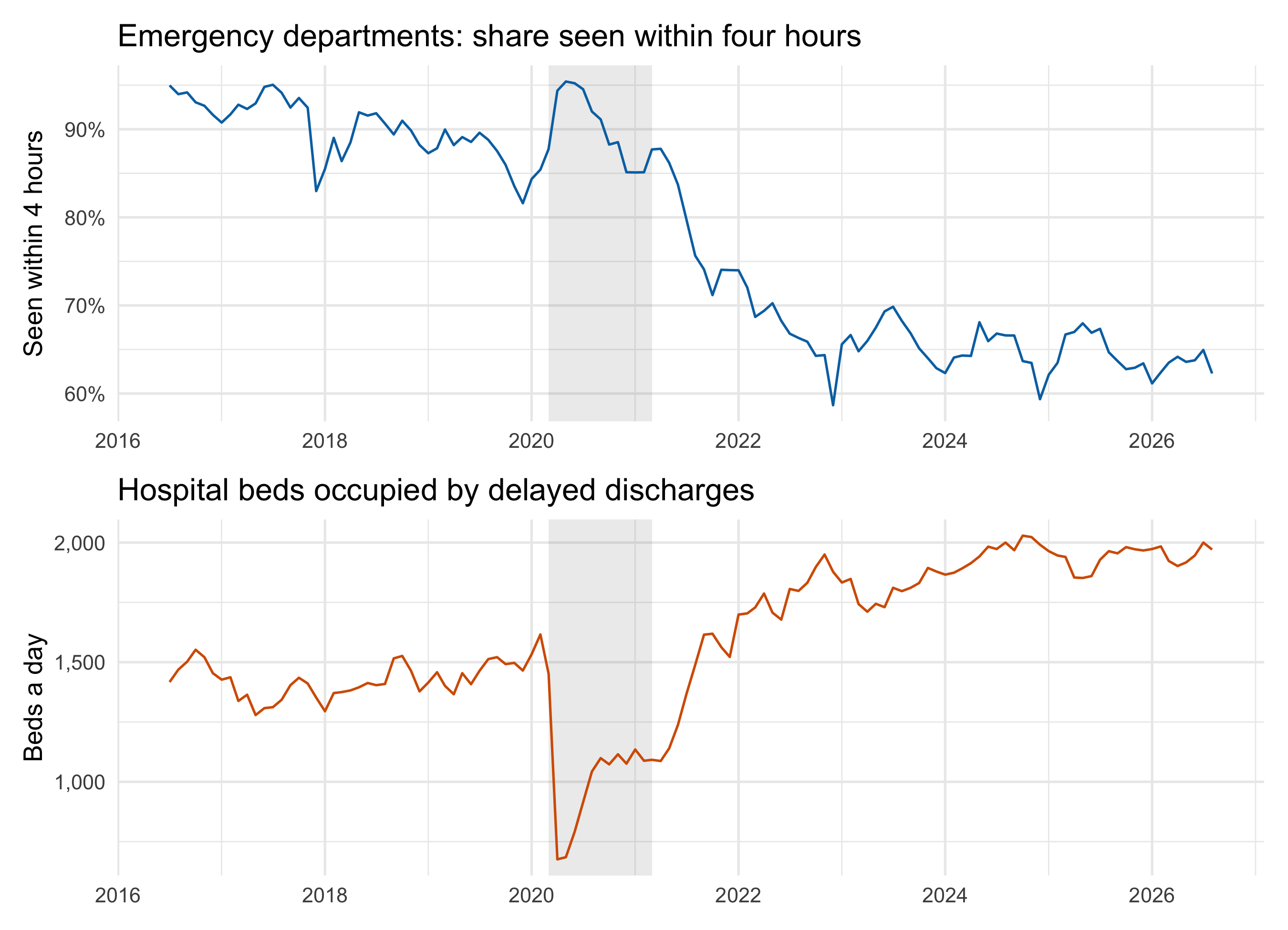
Read one above the other, the two lines look like mirror images. In `r fmt_m(first_m)` emergency departments saw `r pct(at(first_m, "pct_4h"))` of patients within four hours, while delayed discharges took up `r scales::comma(at(first_m, "delayed_beds"))` beds a day. By `r fmt_m(last_m)` the figures were `r pct(at(last_m, "pct_4h"))` and `r scales::comma(at(last_m, "delayed_beds"))`. The pandemic year breaks the pattern in an informative way: delays fell sharply, and four-hour performance briefly recovered with them.
This is how most readers meet the two measures, and it already hints at the relationship. But it asks the reader to do the cross-silo work by eye.
### The cross-silo view: one measure against the other
```{r}
#| label: fig-connected
#| fig-cap: "Scotland, monthly, one point per month joined in time order. Colour runs from the earliest month (dark) to the latest (yellow)."
#| fig-width: 9
#| fig-height: 6.5
both_scot |>
  ggplot(aes(delayed_beds, pct_4h, colour = month)) +
  geom_path(linewidth = 0.5, alpha = 0.6) +
  geom_point(size = 1.8) +
  scale_colour_viridis_c(trans = "date", labels = scales::label_date("%Y")) +
  scale_x_continuous(labels = scales::comma) +
  scale_y_continuous(labels = scales::percent) +
  labs(x = "Beds occupied by delayed discharges (daily average)",
       y = "A&E patients seen within 4 hours", colour = NULL,
       title = "More delayed beds, longer A&E waits") +
  theme_minimal(base_size = 13) +
  theme(legend.key.width = unit(2, "cm"), legend.position = "bottom")
```
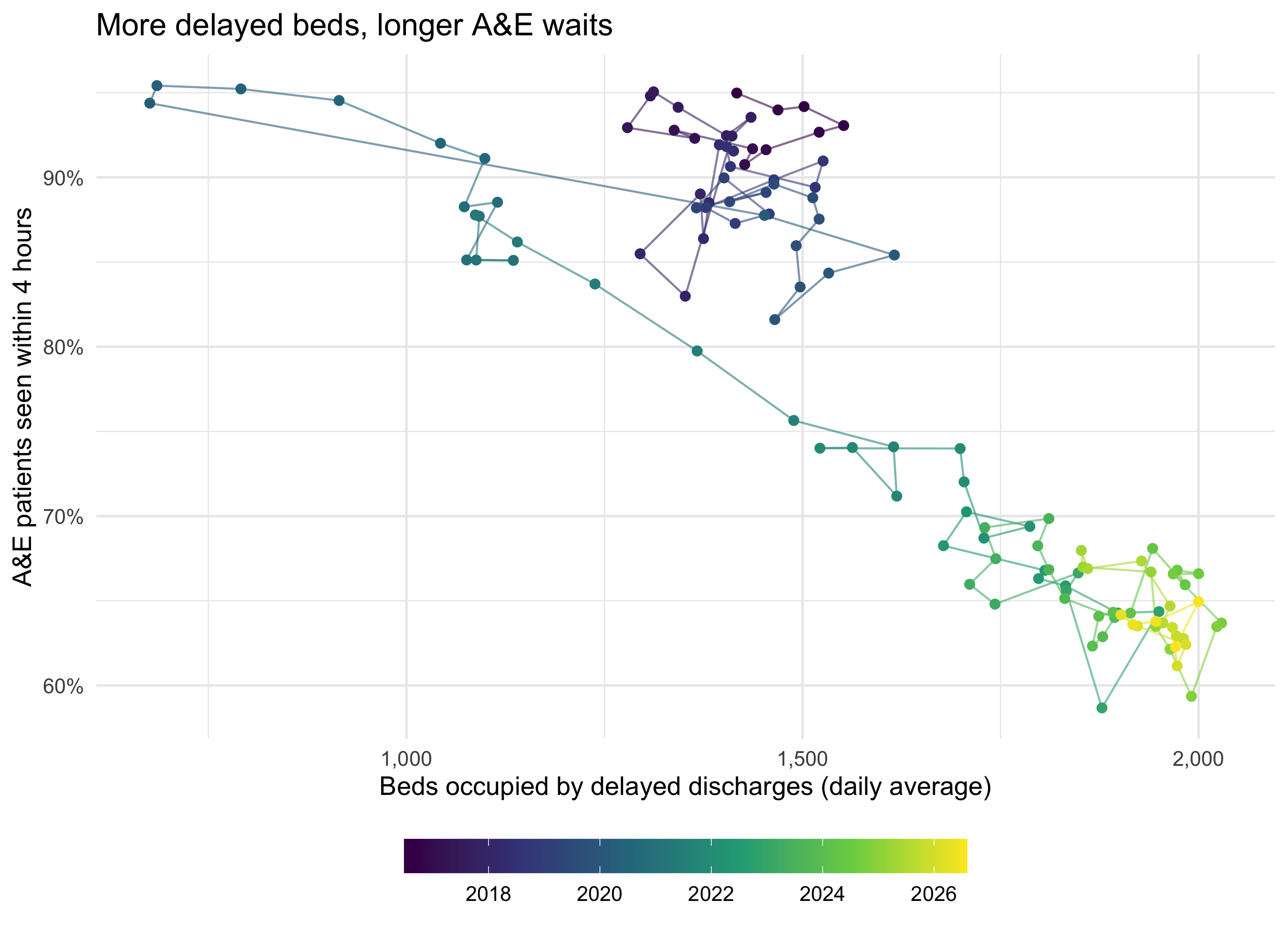
This is the same grammar as the Rosling trails on [the gapminder page](gapminder-fertility.qmd): two measures on x and y, and time carried by the path and the colour. Across the `r nrow(both_scot)` months the correlation is `r round(r_scot, 2)`.
That number needs care. Look inside the dark cluster of pre-pandemic months: it has almost no slope. Most of the correlation comes from the shift between eras, before 2020 and after 2021, not from months with more delays having worse waits. Both series trend over the decade, and almost any two trending series would correlate this strongly. The chart is evidence that the two silos belong on one chart, not evidence that one causes the other. Separating the trend from the month-to-month link is the next question, and probably a session of its own.
### The board view: does every board show it?
```{r}
#| label: fig-boards
#| fig-cap: "Each health board with an emergency department, one point per month, older months fainter. The x scales are free because boards differ hugely in size."
#| fig-width: 9
#| fig-height: 8
both_hb |>
  ggplot(aes(delayed_beds, pct_4h, alpha = month)) +
  geom_point(size = 0.9, colour = "#0072B2") +
  facet_wrap(~ board, scales = "free_x", ncol = 4) +
  scale_x_continuous(n.breaks = 4) +
  scale_alpha_continuous(range = c(0.1, 0.9), trans = "date", guide = "none") +
  scale_y_continuous(labels = scales::percent) +
  labs(x = "Beds occupied by delayed discharges (daily average)",
       y = "A&E patients seen within 4 hours",
       title = "The pattern, board by board") +
  theme_minimal(base_size = 11) +
  theme(panel.spacing.x = unit(1.5, "lines"))
```
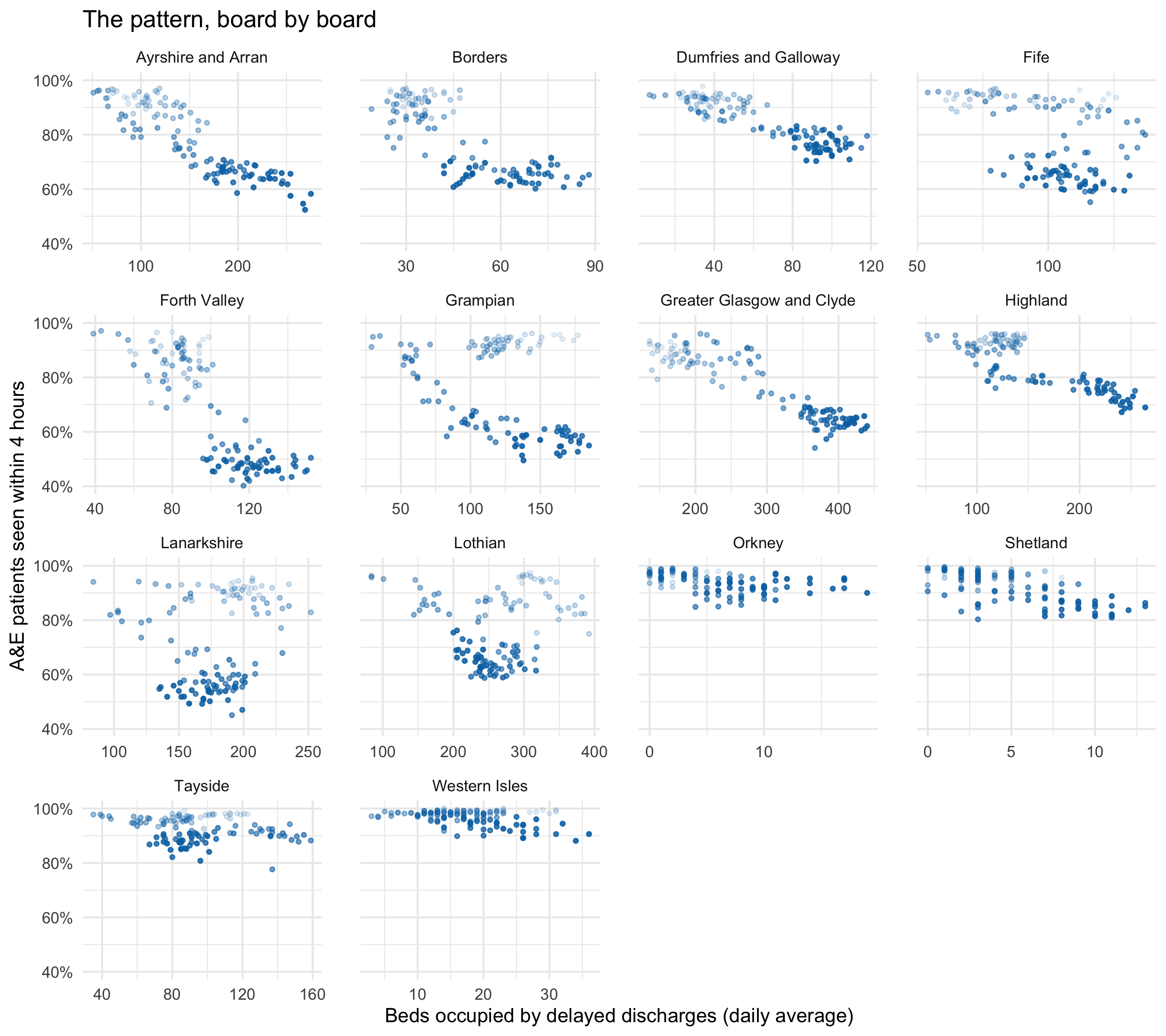
The board panels are where the group's domain knowledge matters most. A board where the cloud slopes clearly down is consistent with exit block. A board where it doesn't is the more interesting case: is it a small island board with few delays to begin with, or a board that kept A&E flowing despite the delays? The data can raise that question but not answer it.
A first look already shows that the boards don't all tell the Scotland story. Ayrshire and Arran, Forth Valley and Greater Glasgow and Clyde slope down much as Scotland does. In Lanarkshire and Lothian, the recent months sit lower than the early ones without sitting further right: A&E performance fell while delays didn't rise, so something other than delayed discharges moved. In Orkney and Shetland, delayed beds are counted in single figures and the points fall into vertical stripes. There, a single patient is a visible step on the x axis.
## Three ways to put two silos on one plot {#three-ways}
The session's grammar exercise is to build the cross-silo chart three ways and compare them.
**1. Vectors from two data frames.** ggplot2 accepts `aes(x = delays_scot$delayed_beds, y = ed_scot$pct_4h)`. This feels like the most direct expression of "this silo against that one", and it needs no join. It's also the fragile one. It pairs rows by position, not by month. The two series here start in different years (`r nrow(ed_scot)` A&E months and `r nrow(delays_scot)` delay months), so this errors, which is the lucky outcome. If the lengths happened to match while the months didn't, it would draw a wrong chart with no warning.
```{r}
#| label: dollar-version
#| eval: false
# Fragile: pairs rows by position, not by month
ggplot() +
  geom_point(aes(x = delays_scot$delayed_beds, y = ed_scot$pct_4h))
```
**2. Each layer with its own data.** For the time-series view, each line can be its own layer with its own `data`, as in the silo figures above. This works whenever the layers share axes, and it is the honest version of "one plot, several silos". It can't make a scatter of one silo against the other, because a point needs both values in one row.
**3. Join on the shared keys, then plot.** `inner_join(ed_scot, delays_scot, by = "month")` is what this page does. The join makes the pairing rule explicit and checkable: the same board, the same month. It also drops months that only one silo has, and the validator can check what was dropped.
The comparison is the lesson. The grammar allows all three. Choosing between them is about how errors are kept out, and that is the validator's job, not the coder's.
## Candidate mappings (the group chooses)
``` text
Candidates (the group chooses) - nhs-cross-silo:
  joined grain:   board x month (14 boards with an ED, Jul 2016 - Aug 2026)
  position x/y:   pct_4h (A&E), delayed_beds (delays), month (time)
  time:           month - as x, as path order, as colour, or as alpha
  facet:          board (14) - free scales needed; or year
  colour:         year or season (winter vs rest) - not board (too many)
  size:           attendances (board size) - but it dominates, as population did in gapminder
  other silos:    attendances (demand), delay reason (health/social care vs Code 9)
```
Questions for the group:
- **Rates or counts?** Delayed beds are a count, and boards differ in size by an order of magnitude. Beds per 100,000 adults would need a third, population, silo.
- **Season.** Winter pressure moves both measures together. Colour by season, or facet by year, to see whether the link holds outside winter.
- **The third silo.** Ambulance handover times would complete the chain from front door to back door. They aren't on the Public Health Scotland open data portal (as of 2026-10-09 the only ambulance dataset there is from a COVID-19 wider-impacts series). Finding a public source is a task worth setting before the session.
## What the data can't say
These are monthly board totals, so they can't follow a patient. They can't show that the person waiting in A&E was waiting for the bed that a delayed patient occupied. Both measures share drivers, such as an ageing population, winter, the pandemic and staffing, that could move them together without one causing the other. The four-hour figure counts all Type 1 attendances, including the majority who are never admitted and so never need a ward bed. A cleaner test would use admitted patients only, and that breakdown isn't in this file. The delayed-discharge figures come from a monthly census and bed-day returns, with definitions set nationally. A change in what counts as a delay would show up as a change in the line. Finally, the joined record covers about ten years, which includes one pandemic and very few independent "experiments".