The Office: what’s in the data

Session 1 · TidyTuesday 2020-03-17 · Grammar layer: data & aesthetic mappings

TipSession 1 · 2026-09-29 · facilitated by Jon Minton

With six or seven participants, two in the room and the rest joining remotely. No one is named, because no consent record was taken. Design decisions were made live by the group. This page is the workbook as it stood at the end of the session, prepared by Claude Opus 5.5 from the spec files and figures, with reflections added by the facilitator. The session was not recorded, and the page was approved before publishing. How these sessions work.

TidyTuesday for 2020-03-17 covers the US version of The Office (NBC, 2005–2013). The week itself ships one table, IMDb ratings per episode, and points to the schrute R package for the full dialogue. Both are described here.

TipReproducing this page

Runs from two CSVs cached in data/. The ratings CSV is committed in this repository. The transcripts CSV holds the show’s full dialogue, so it is not committed; the second block below rebuilds it locally. To refresh from source:

# IMDb ratings: the TidyTuesday week
download.file(
  "https://raw.githubusercontent.com/rfordatascience/tidytuesday/main/data/2020/2020-03-17/office_ratings.csv",
  "data/tt-2020-03-17-office_ratings.csv")

# Transcripts: the schrute package's data, read without installing the package
tmp <- tempfile(fileext = ".rda")
download.file(
  "https://raw.githubusercontent.com/bradlindblad/schrute/master/data/theoffice.rda",
  tmp, mode = "wb")
load(tmp)
readr::write_csv(theoffice, "data/schrute-theoffice.csv")

Packages: tidyverse. Sources: IMDb ratings via data.world; transcripts via Brad Lindblad’s schrute package (MIT), from fan transcriptions; both through TidyTuesday 2020-03-17.

library(tidyverse)

ratings <- read_csv("../../data/tt-2020-03-17-office_ratings.csv", show_col_types = FALSE)
lines   <- read_csv("../../data/schrute-theoffice.csv", show_col_types = FALSE)

n_ep_lines   <- n_distinct(lines$season, lines$episode)
n_characters <- n_distinct(lines$character)
top_speakers <- lines |> count(character, sort = TRUE) |> slice_head(n = 5)

At a glance

Table	Grain	Rows × columns
office_ratings	one row per episode	188 × 6
theoffice (schrute)	one row per spoken line	55,130 × 12

The two tables share season and episode, which is the join key. The transcript table already carries the IMDb rating, vote count and air date on every line, so it is effectively a line-level table with episode-level columns repeated on each row.

office_ratings: one row per episode

188 episodes across 9 seasons, aired between March 2005 and May 2013. IMDb ratings run from 6.7 to 9.7, and vote counts from 1,393 to 7,934. There are no missing values.

head(ratings)

season	episode	title	imdb_rating	total_votes	air_date
1	1	Pilot	7.6	3706	2005-03-24
1	2	Diversity Day	8.3	3566	2005-03-29
1	3	Health Care	7.9	2983	2005-04-05
1	4	The Alliance	8.1	2886	2005-04-12
1	5	Basketball	8.4	3179	2005-04-19
1	6	Hot Girl	7.8	2852	2005-04-26

Variable	Type (grammar terms)	Notes
season	discrete* (9 levels)	whole numbers, so whether it is discrete or continuous is a decision
episode	continuous, or ordinal within season	numbering restarts each season
title	identifier	a label, not an aesthetic
imdb_rating	continuous	10 is best
total_votes	continuous	IMDb users who rated the episode
air_date	temporal	original US air date

theoffice: one row per spoken line

55,130 lines of dialogue from 186 episodes, spoken by 769 distinct character labels. The most frequent speakers are Michael (10,924), Dwight (6,849), Jim (6,305), Pam (5,032), Andy (3,754).

lines |>
  mutate(across(c(text, text_w_direction, writer), \(x) str_trunc(x, 40))) |>
  head()

index	season	episode	episode_name	director	writer	character	text	text_w_direction	imdb_rating	total_votes	air_date
1	1	1	Pilot	Ken Kwapis	Ricky Gervais;Stephen Merchant;Greg D…	Michael	All right Jim. Your quarterlies look …	All right Jim. Your quarterlies look …	7.6	3706	2005-03-24
2	1	1	Pilot	Ken Kwapis	Ricky Gervais;Stephen Merchant;Greg D…	Jim	Oh, I told you. I couldn’t close it. …	Oh, I told you. I couldn’t close it. …	7.6	3706	2005-03-24
3	1	1	Pilot	Ken Kwapis	Ricky Gervais;Stephen Merchant;Greg D…	Michael	So you’ve come to the master for guid…	So you’ve come to the master for guid…	7.6	3706	2005-03-24
4	1	1	Pilot	Ken Kwapis	Ricky Gervais;Stephen Merchant;Greg D…	Jim	Actually, you called me in here, but …	Actually, you called me in here, but …	7.6	3706	2005-03-24
5	1	1	Pilot	Ken Kwapis	Ricky Gervais;Stephen Merchant;Greg D…	Michael	All right. Well, let me show you how …	All right. Well, let me show you how …	7.6	3706	2005-03-24
6	1	1	Pilot	Ken Kwapis	Ricky Gervais;Stephen Merchant;Greg D…	Michael	Yes, I’d like to speak to your office…	[on the phone] Yes, I’d like to speak…	7.6	3706	2005-03-24

Variable	Type (grammar terms)	Notes
index	identifier / order	running line number across the whole series
season, episode, episode_name	discrete	the join key back to office_ratings
director, writer	discrete (many levels)	writer can hold several names separated by ;
character	discrete (769 levels)	far too many for colour. Filter or lump first
text, text_w_direction	free text	the second keeps stage directions in brackets
imdb_rating, total_votes, air_date	as above	repeated on every line of an episode

A first figure: ratings by season and episode

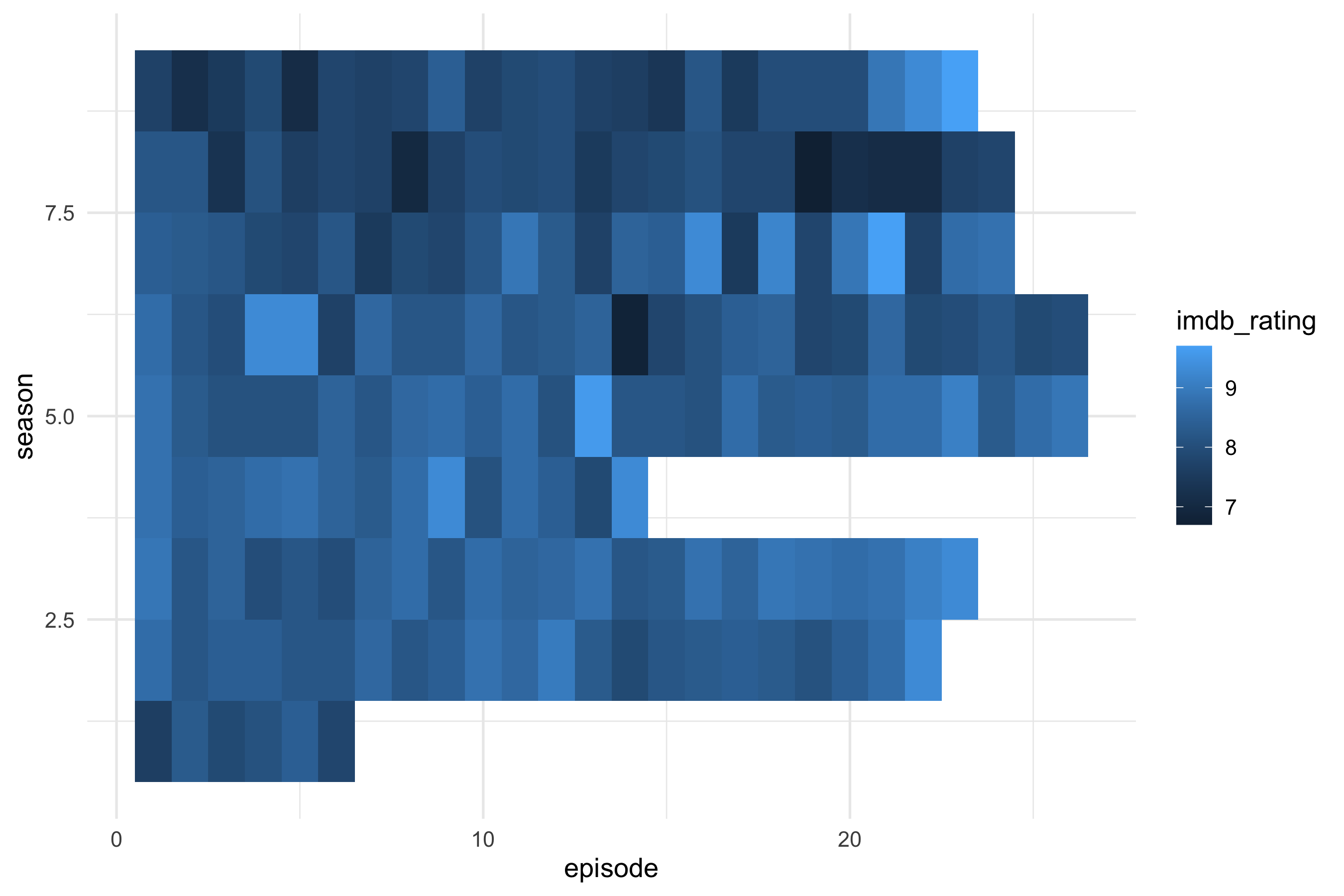
The first spec asked for a heatmap: season as rows, episode number as columns, and IMDb rating as fill. Everything else is left at ggplot2’s defaults.

# sessions/2026-09-29/specs/01-office-heatmap.yml
data: tt-2020-03-17-office_ratings
mapping:
  x: episode
  y: season
  fill: imdb_rating
layers:
  - geom: tile

ggplot(ratings, aes(x = episode, y = season, fill = imdb_rating)) +
  geom_tile() +
  theme_minimal(base_size = 13)

Figure 1

Looking at the render shows three defaults that nobody decided on:

• season is stored as a number, so ggplot2 treats it as continuous. The axis shows breaks at 2.5, 5.0 and 7.5, which are seasons that don’t exist.
• The default continuous y scale puts season 1 at the bottom and season 9 at the top.
• The default fill gradient runs from dark to light blue, which leaves little contrast across the 6.7–9.7 range.

The ragged right edge shows how many episodes each season had. Season 1 is the shortest, with 6 episodes.

A second figure: ratings over air date

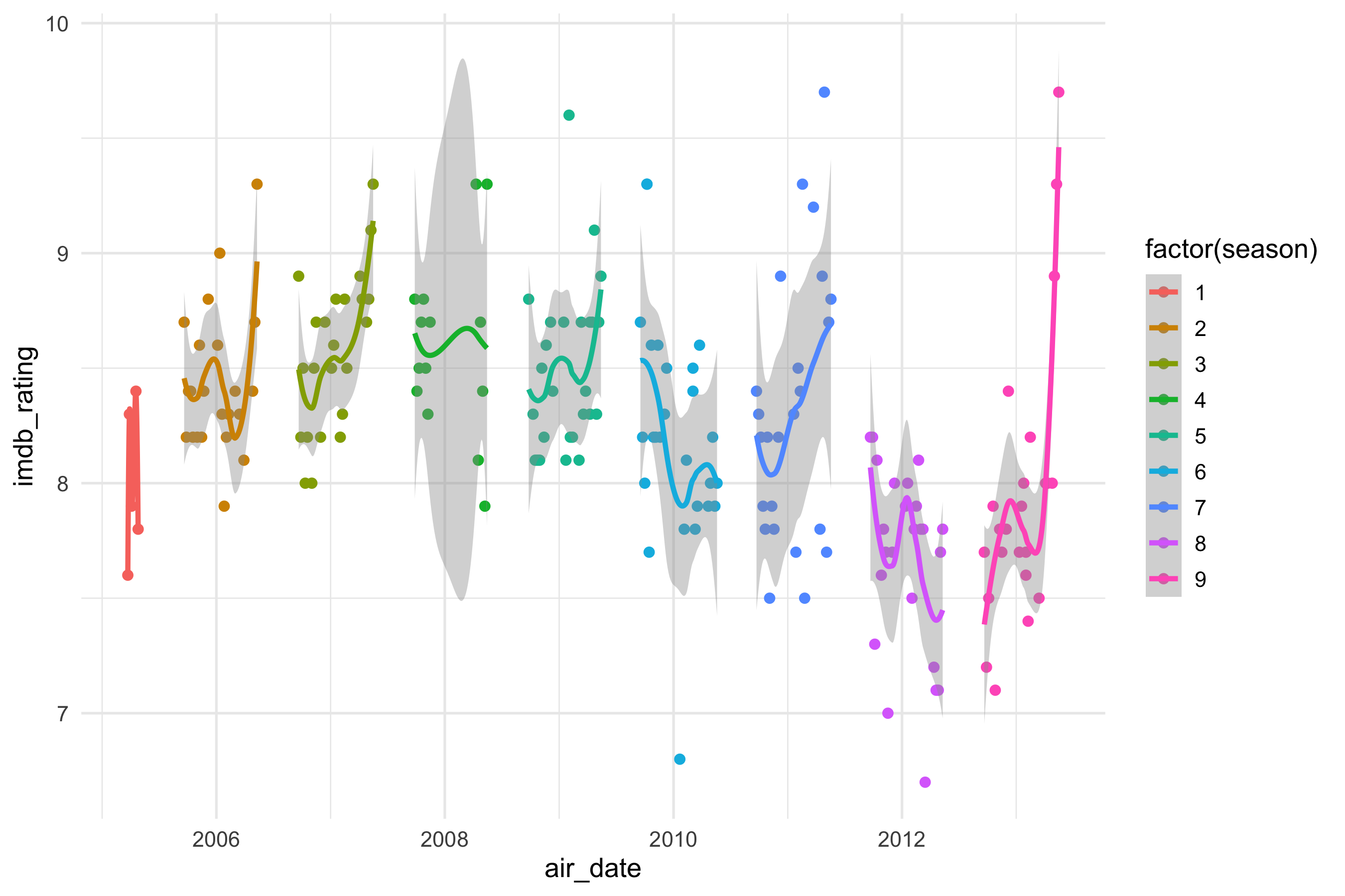
The second spec puts each episode at its air date, colours it by season, and adds a smoother. Two decisions were made before compiling:

• Season as a category. season is stored as a number, so the spec maps factor(season) to colour, which gives one hue per season instead of a gradient. Shape was dropped: ggplot2’s default shape palette has only six shapes, so seasons 7–9 would have gone missing.
• One smoother per season. Colour is mapped for the whole plot, so the smooth layer inherits it and fits a separate curve to each season.

# sessions/2026-09-29/specs/02-office-airdate.yml
data: tt-2020-03-17-office_ratings
mapping:
  x: air_date
  y: imdb_rating
  colour: factor(season)
layers:
  - geom: point
  - geom: smooth

ggplot(ratings, aes(x = air_date, y = imdb_rating, colour = factor(season))) +
  geom_point() +
  geom_smooth() +
  theme_minimal(base_size = 13)

Figure 2

Looking at the render:

• The smoother defaults to loess, which is very wiggly when seasons are this short (a median of 23 episodes). Season 1’s 6 episodes give a spike with no confidence ribbon, and R prints a warning while fitting it.
• Season 4’s ribbon balloons across a gap in its air dates. Loess is drawing a curve through months with no episodes.
• Several seasons end on a rise, most sharply the finale at 9.7. A flexible smoother bends towards the last point or two, so these end-of-season spikes need checking against the raw points before reading anything into them.
• The legend title is the code factor(season), and the axis titles are raw variable names, because the spec has no labs block yet.

What the data can’t say

IMDb ratings come from self-selected raters voting years after broadcast, so they measure how the show is remembered by people who chose to rate it. They don’t measure how it was received at the time. The episode counts also differ between tables (188 rated episodes against 186 in the transcripts). The sources likely split two-part episodes differently. Check any join for dropped rows. The transcripts are fan-made, so character labels are inconsistent: the same person can appear under several spellings, which inflates the character count.

Reflections on in-person/hybrid session

• Some people had preference for something more GUI/point-and-click rather than the dev-style IDE presented.

  • My discussion about text-based ragged data structures, like the YAML/JSON-like universal gg specification offered in the gg-spec skill, might have been too close to the bedrock on average.

• Less resistance to CC/Codex taking over implementation tasks than I was expecting.

• Soft support for key argument made: that more of analysts/analytical knowledge workers’ time should be spent on the design decisions.

  • e.g. I mentioned ggplot2 used to have qplot, but the defaults took too many important design decisions from the user, so was deprecated.

  • This is now the ‘stuff to sweat’, though maybe a gui will help even more

• Less continual iteration over specific visualisation. Didn’t get to show committing as like rappeling in rock climbing, and this being an organic process.

Next steps:

• Get workbook at the end of the session committed and rendered as a page on github pages for showing to attendees.

• Get a second version of the workshop doc with incremental improvements to visualisation also shown, along with a ‘wow’ visualisation’, such as a 3D plot, and something generated by Opus 5.5 autonomously.

• Produce a skill with replicates a tableau-style gui way of specifying mapping from dataset features to visual aesthetics in a ggplot2 way. Have this as another page along with some ready datasets to select from.

• Contextualise what the workshop showed as one key aspect of one of the three modules I’m developing for the Knowledge Tree collection, namely ‘Science Supercharged’. Give links and a description to the broader package and illustrative savings in total time through collapsing of implementation time.