---
title: "The Office: what's in the data, version 2"
subtitle: "Session 1, continued · TidyTuesday 2020-03-17 · Grammar layer: data & aesthetic mappings"
date: 2026-10-01
---
::: {.callout-tip icon="false"}
## Session 1 · 2026-09-29 · facilitated by Jon Minton · version 2
This page begins exactly as the [end-of-session workbook](office-data.qmd) does, then continues past it. Everything above the line marked **Version 2 begins here** is the workbook as the group left it. Everything below it was made after the session:
- the revised specs (03–05) follow the facilitator's decisions
- the facilitator specified the 3D figure and its models
- one section was produced autonomously by Claude Opus 5.5 and is labelled as such
No participant is named, because no consent record was taken. [How these sessions work](../../index.qmd).
:::
TidyTuesday for 2020-03-17 covers the US version of *The Office* (NBC, 2005–2013). The week itself ships one table, IMDb ratings per episode, and points to the [`schrute`](https://bradlindblad.github.io/schrute/) R package for the full dialogue. Both are described here.
::: {.callout-tip collapse="true"}
## Reproducing this page
Runs from two CSVs cached in `data/`. The ratings CSV is committed in this repository. The transcripts CSV holds the show's full dialogue, so it is not committed; the second block below rebuilds it locally. To refresh from source:
``` r
# IMDb ratings: the TidyTuesday week
download.file(
  "https://raw.githubusercontent.com/rfordatascience/tidytuesday/main/data/2020/2020-03-17/office_ratings.csv",
  "data/tt-2020-03-17-office_ratings.csv")

# Transcripts: the schrute package's data, read without installing the package
tmp <- tempfile(fileext = ".rda")
download.file(
  "https://raw.githubusercontent.com/bradlindblad/schrute/master/data/theoffice.rda",
  tmp, mode = "wb")
load(tmp)
readr::write_csv(theoffice, "data/schrute-theoffice.csv")
```
Packages: `tidyverse`. Sources: IMDb ratings via [data.world](https://data.world/anujjain7/the-office-imdb-ratings-dataset); transcripts via Brad Lindblad's [`schrute`](https://github.com/bradlindblad/schrute) package (MIT), from fan transcriptions; both through TidyTuesday [2020-03-17](https://github.com/rfordatascience/tidytuesday/tree/main/data/2020/2020-03-17).
:::
```{r setup}
library(tidyverse)

ratings <- read_csv("../../data/tt-2020-03-17-office_ratings.csv", show_col_types = FALSE)
lines   <- read_csv("../../data/schrute-theoffice.csv", show_col_types = FALSE)

n_ep_lines   <- n_distinct(lines$season, lines$episode)
n_characters <- n_distinct(lines$character)
top_speakers <- lines |> count(character, sort = TRUE) |> slice_head(n = 5)
```
## At a glance
| Table | Grain | Rows × columns |
|------------------------|------------------------|------------------------|
| `office_ratings` | one row per episode | `r nrow(ratings)` × `r ncol(ratings)` |
| `theoffice` (schrute) | one row per spoken line | `r format(nrow(lines), big.mark = ",")` × `r ncol(lines)` |
The two tables share `season` and `episode`, which is the join key. The transcript table already carries the IMDb rating, vote count and air date on every line, so it is effectively a line-level table with episode-level columns repeated on each row.
## `office_ratings`: one row per episode
`r nrow(ratings)` episodes across `r n_distinct(ratings$season)` seasons, aired between `r format(min(ratings$air_date), "%B %Y")` and `r format(max(ratings$air_date), "%B %Y")`. IMDb ratings run from `r min(ratings$imdb_rating)` to `r max(ratings$imdb_rating)`, and vote counts from `r format(min(ratings$total_votes), big.mark = ",")` to `r format(max(ratings$total_votes), big.mark = ",")`. There are no missing values.
```{r ratings-head}
head(ratings)
```
| Variable | Type (grammar terms) | Notes |
|------------------------|------------------------|------------------------|
| `season` | discrete\* (`r n_distinct(ratings$season)` levels) | whole numbers, so whether it is discrete or continuous is a decision |
| `episode` | continuous, or ordinal within season | numbering restarts each season |
| `title` | identifier | a label, not an aesthetic |
| `imdb_rating` | continuous | 10 is best |
| `total_votes` | continuous | IMDb users who rated the episode |
| `air_date` | temporal | original US air date |
## `theoffice`: one row per spoken line
`r format(nrow(lines), big.mark = ",")` lines of dialogue from `r n_ep_lines` episodes, spoken by `r n_characters` distinct character labels. The most frequent speakers are `r paste0(top_speakers$character, " (", format(top_speakers$n, big.mark = ",", trim = TRUE), ")", collapse = ", ")`.
```{r lines-head}
lines |>
  mutate(across(c(text, text_w_direction, writer), \(x) str_trunc(x, 40))) |>
  head()
```
| Variable | Type (grammar terms) | Notes |
|------------------------|------------------------|------------------------|
| `index` | identifier / order | running line number across the whole series |
| `season`, `episode`, `episode_name` | discrete | the join key back to `office_ratings` |
| `director`, `writer` | discrete (many levels) | `writer` can hold several names separated by `;` |
| `character` | discrete (`r n_characters` levels) | far too many for colour. Filter or lump first |
| `text`, `text_w_direction` | free text | the second keeps stage directions in brackets |
| `imdb_rating`, `total_votes`, `air_date` | as above | repeated on every line of an episode |
## A first figure: ratings by season and episode
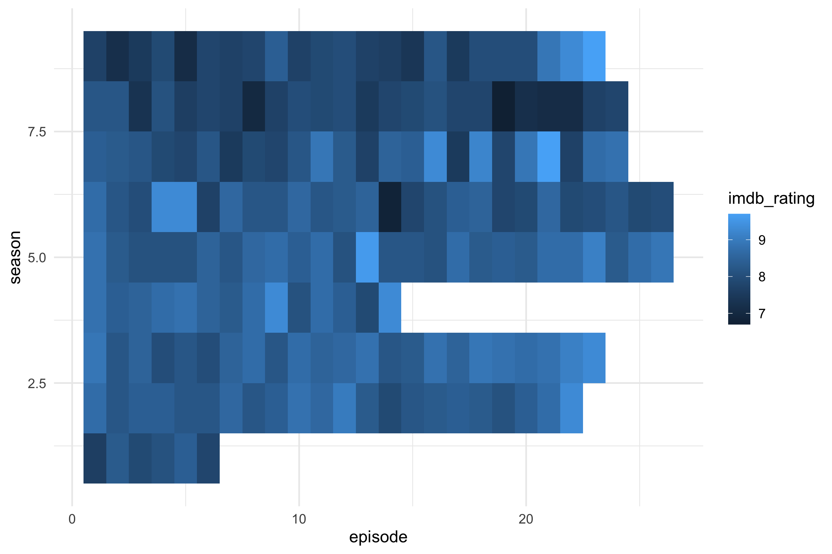
The first spec asked for a heatmap: season as rows, episode number as columns, and IMDb rating as fill. Everything else is left at ggplot2's defaults.
``` yaml
# sessions/2026-09-29/specs/01-office-heatmap.yml
data: tt-2020-03-17-office_ratings
mapping:
  x: episode
  y: season
  fill: imdb_rating
layers:
  - geom: tile
```
```{r fig-heatmap}
#| fig-alt: "Heatmap of IMDb rating for each episode of The Office, seasons as rows and episode number as columns."
ggplot(ratings, aes(x = episode, y = season, fill = imdb_rating)) +
  geom_tile() +
  theme_minimal(base_size = 13)
```
Looking at the render shows three defaults that nobody decided on:
- `season` is stored as a number, so ggplot2 treats it as continuous. The axis shows breaks at 2.5, 5.0 and 7.5, which are seasons that don't exist.
- The default continuous y scale puts season 1 at the bottom and season 9 at the top.
- The default fill gradient runs from dark to light blue, which leaves little contrast across the `r min(ratings$imdb_rating)`–`r max(ratings$imdb_rating)` range.
The ragged right edge shows how many episodes each season had. Season `r ratings |> count(season) |> slice_min(n, n = 1, with_ties = FALSE) |> pull(season)` is the shortest, with `r ratings |> count(season) |> pull(n) |> min()` episodes.
## A second figure: ratings over air date
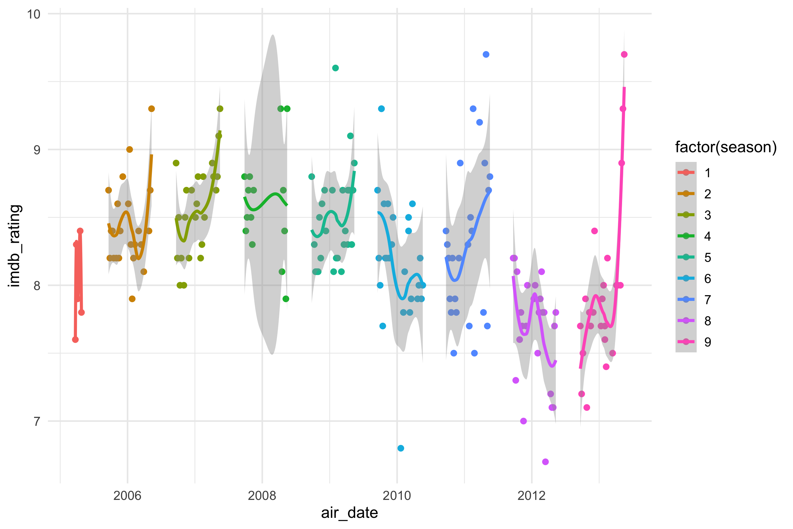
The second spec puts each episode at its air date, colours it by season, and adds a smoother. Two decisions were made before compiling:
- **Season as a category.** `season` is stored as a number, so the spec maps `factor(season)` to colour, which gives one hue per season instead of a gradient. Shape was dropped: ggplot2's default shape palette has only six shapes, so seasons 7–9 would have gone missing.
- **One smoother per season.** Colour is mapped for the whole plot, so the smooth layer inherits it and fits a separate curve to each season.
``` yaml
# sessions/2026-09-29/specs/02-office-airdate.yml
data: tt-2020-03-17-office_ratings
mapping:
  x: air_date
  y: imdb_rating
  colour: factor(season)
layers:
  - geom: point
  - geom: smooth
```
```{r fig-airdate}
#| fig-alt: "IMDb rating of each episode of The Office against air date, coloured by season, with a separate smoother for each season."
ggplot(ratings, aes(x = air_date, y = imdb_rating, colour = factor(season))) +
  geom_point() +
  geom_smooth() +
  theme_minimal(base_size = 13)
```
Looking at the render:
- The smoother defaults to loess, which is very wiggly when seasons are this short (a median of `r ratings |> count(season) |> pull(n) |> median()` episodes). Season 1's `r sum(ratings$season == 1)` episodes give a spike with no confidence ribbon, and R prints a warning while fitting it.
- Season 4's ribbon balloons across a gap in its air dates. Loess is drawing a curve through months with no episodes.
- Several seasons end on a rise, most sharply the finale at `r max(ratings$imdb_rating)`. A flexible smoother bends towards the last point or two, so these end-of-season spikes need checking against the raw points before reading anything into them.
- The legend title is the code `factor(season)`, and the axis titles are raw variable names, because the spec has no `labs` block yet.
---
# Version 2 begins here
Everything from here on was made after the session.
```{r v2-setup}
library(plotly)
library(broom)

season_cols <- scales::hue_pal()(9)   # the same hues ggplot2 gave the seasons above
```
## Revisions to the first two figures
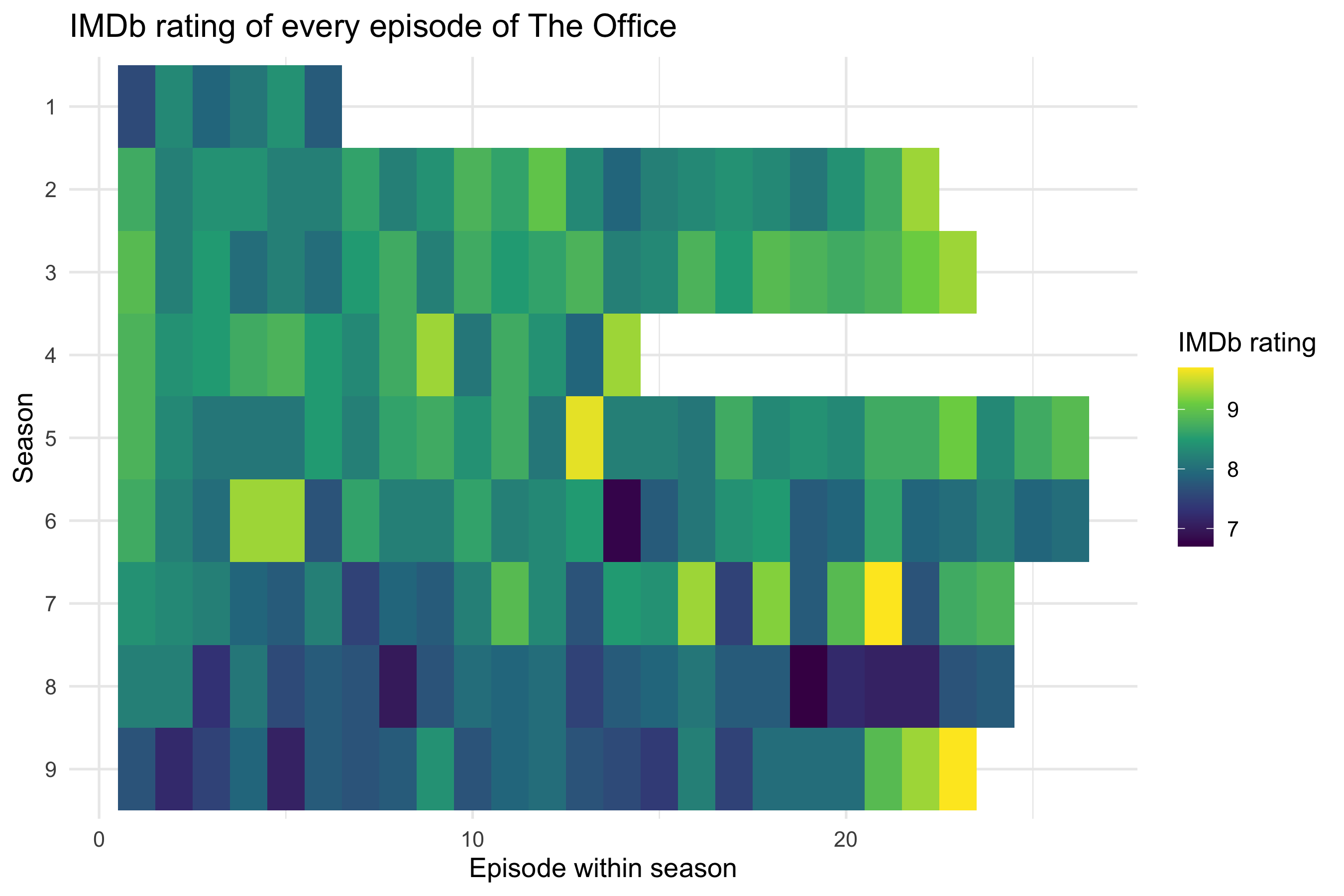
The facilitator reviewed what the renders had revealed and made these decisions:
- Season is a **category**, not a cardinal number. Season 3 isn't "three times" season 1.
- Season 1 goes at the top, so the heatmap reads like a table.
- The fill uses viridis for more contrast across the ratings.
- Per-season smoothers become straight lines (`method: lm`).
- A second version shows one smoother for the whole series.
- Every figure gets proper labels.
### Spec 03: the heatmap, revised
``` yaml
# sessions/2026-09-29/specs/03-office-heatmap-v2.yml
data: tt-2020-03-17-office_ratings
mapping:
  x: episode
  y: factor(season)
  fill: imdb_rating
layers:
  - geom: tile
scales:
  y: scale_y_discrete(limits = rev)
  fill: viridis
labs:
  title: "IMDb rating of every episode of The Office"
  x: "Episode within season"
  y: "Season"
  fill: "IMDb rating"
```
```{r fig-heatmap-v2}
#| fig-alt: "Heatmap of IMDb ratings with seasons 1 to 9 as discrete rows from top to bottom, episodes as columns, and a viridis fill."
ggplot(ratings, aes(x = episode, y = factor(season), fill = imdb_rating)) +
  geom_tile() +
  scale_y_discrete(limits = rev) +
  scale_fill_viridis_c() +
  labs(title = "IMDb rating of every episode of The Office",
       x = "Episode within season", y = "Season", fill = "IMDb rating") +
  theme_minimal(base_size = 13)
```
With season as a category, each row is one season and the axis shows only seasons that exist. `scale_y_discrete(limits = rev)` puts season 1 at the top. Viridis runs from dark purple to yellow, so the season 8 slump and the high points stand out. The finale is the brightest tile in the last row.
### Spec 04: one straight line per season
``` yaml
# sessions/2026-09-29/specs/04-office-airdate-lm.yml
data: tt-2020-03-17-office_ratings
mapping:
  x: air_date
  y: imdb_rating
  colour: factor(season)
layers:
  - geom: point
  - geom: smooth
    method: lm
labs:
  title: "Ratings over the run, with a linear trend per season"
  x: "Original air date"
  y: "IMDb rating"
  colour: "Season"
```
```{r fig-airdate-lm}
#| fig-alt: "IMDb rating against air date, coloured by season, with a straight regression line and confidence band for each season."
ggplot(ratings, aes(x = air_date, y = imdb_rating, colour = factor(season))) +
  geom_point() +
  geom_smooth(method = "lm") +
  labs(title = "Ratings over the run, with a linear trend per season",
       x = "Original air date", y = "IMDb rating", colour = "Season") +
  theme_minimal(base_size = 13)
```
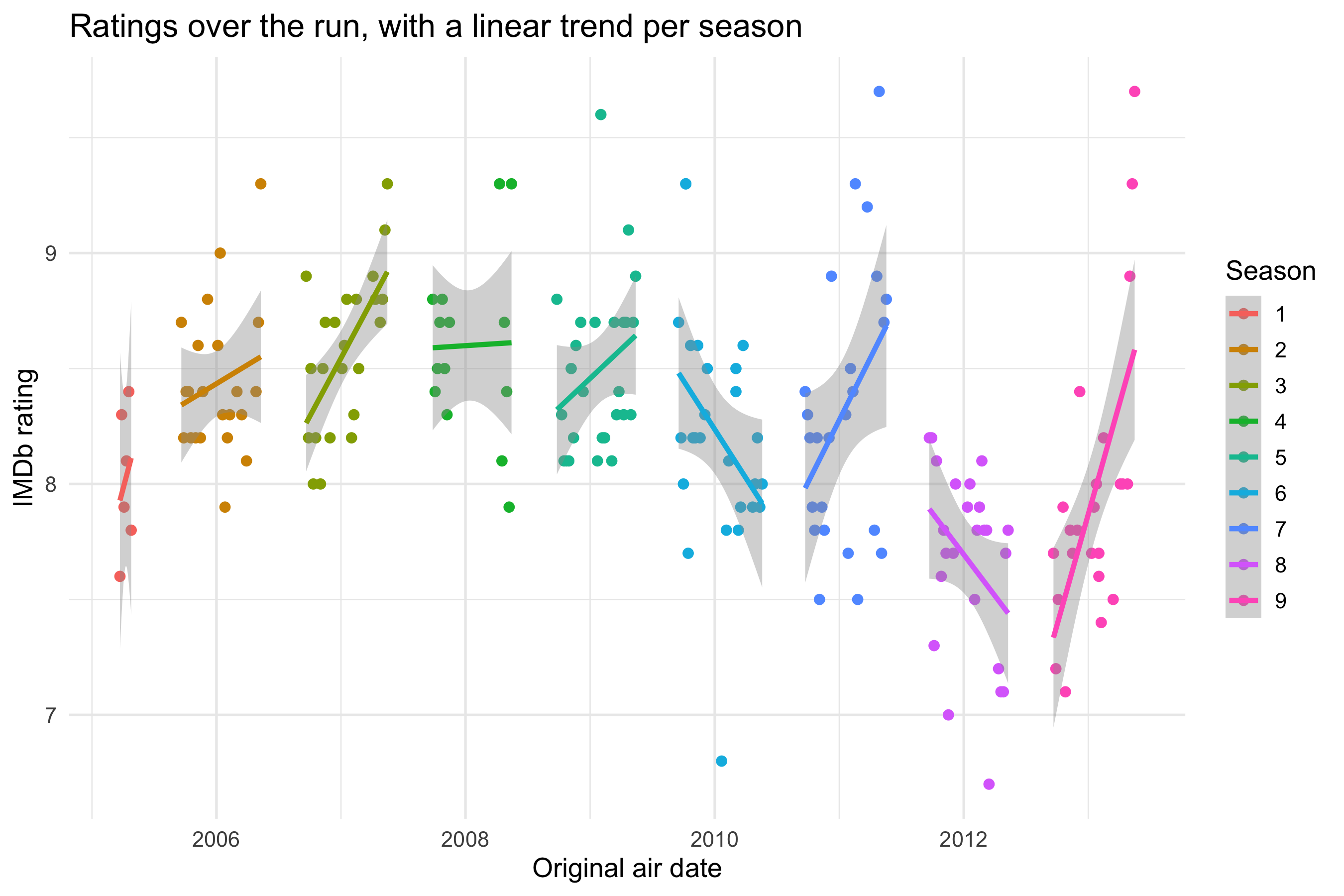
`geom_smooth(method = "lm")` runs a regression that doesn't appear anywhere in the code. For each season, ggplot2 fits `lm(imdb_rating ~ air_date)` to that season's episodes and draws the fitted line with a 95% confidence band. The straight lines are far steadier than the loess curves of the first version. Season 4's line now crosses its gap in air dates without bending. That gap is still worth knowing about: a line drawn through months with no episodes claims nothing about them.
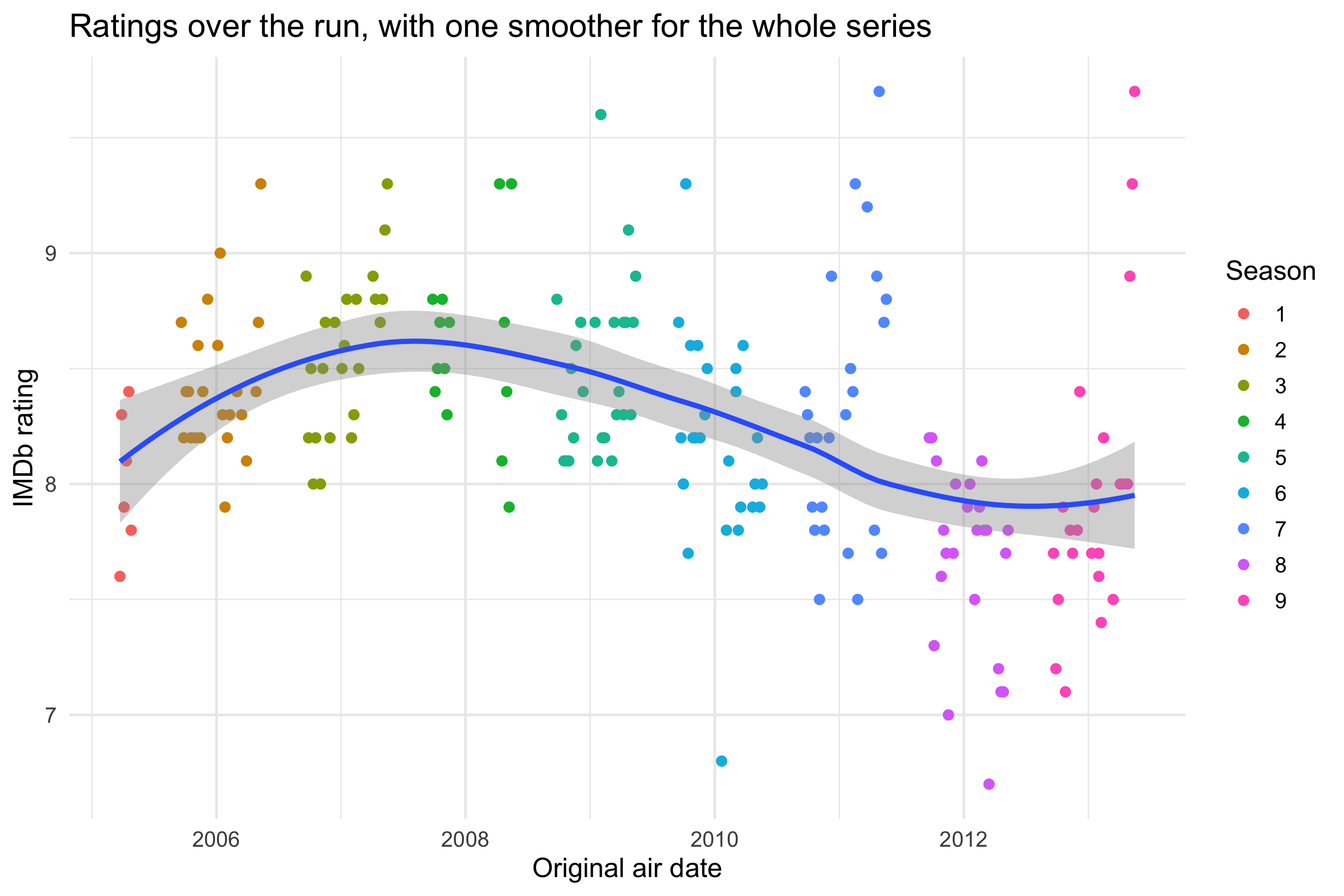
### Spec 05: one smoother for the whole series
This spec uses a feature that was added to the gg-spec schema for it: a **layer-level mapping**. Colour is mapped on the point layer only, so the smooth layer no longer inherits it and fits one curve to all `r nrow(ratings)` episodes.
``` yaml
# sessions/2026-09-29/specs/05-office-airdate-pooled.yml
data: tt-2020-03-17-office_ratings
mapping:
  x: air_date
  y: imdb_rating
layers:
  - geom: point
    mapping:
      colour: factor(season)
  - geom: smooth
labs:
  title: "Ratings over the run, with one smoother for the whole series"
  x: "Original air date"
  y: "IMDb rating"
  colour: "Season"
```
```{r fig-airdate-pooled}
#| fig-alt: "IMDb rating against air date with points coloured by season and a single loess smoother rising to a peak around 2007 and declining afterwards."
ggplot(ratings, aes(x = air_date, y = imdb_rating)) +
  geom_point(aes(colour = factor(season))) +
  geom_smooth() +
  labs(title = "Ratings over the run, with one smoother for the whole series",
       x = "Original air date", y = "IMDb rating", colour = "Season") +
  theme_minimal(base_size = 13)
```
Moving one `colour` mapping from the plot level to the point layer changes the question the figure answers. Spec 04 asks how ratings move *within* a season. Spec 05 asks how they move across the whole run: up to a peak in seasons 3 and 4, then down. With `r nrow(ratings)` points, loess is no longer too flexible.
## A 3D view, with the models made explicit
```{r models}
# Within-season lines: season as a category, with its own intercept and slope.
# This parameterisation gives each season's intercept and slope directly.
m_lines <- lm(imdb_rating ~ 0 + factor(season) + factor(season):episode, data = ratings)

# Across-season planes: season as a cardinal number.
m_plane <- lm(imdb_rating ~ episode + season, data = ratings)   # flat plane
m_twist <- lm(imdb_rating ~ episode * season, data = ratings)   # twisted plane

r2 <- \(m) sprintf("%.2f", summary(m)$r.squared)

# Comparable R² for the within-season model: refit it with an intercept (same fitted
# values, same residuals) so R² is measured against the mean rating, not against zero.
r2_lines <- summary(lm(imdb_rating ~ factor(season) * episode, data = ratings))$r.squared
```
Rating is elevation, episode is x and season is y. Use the buttons to add one of three linear models. The table alongside updates to show the model behind the surface, its `lm()` call, and its coefficients. Drag to rotate the view, and scroll to zoom.
Seen from straight above, this is the heatmap again, with rating as height instead of colour.
The buttons offer two kinds of model:
- **Within-season lines** treat season as a category, as the facilitator decided. Each season gets its own intercept and slope, so this is the model that spec 04's `geom_smooth(method = "lm")` fits implicitly. The one difference is that x here is episode number, where spec 04 used air date.
- **Across-season planes** treat season as a **cardinal** number. That goes against the decision above, and it has to: a plane needs a continuous y. Season becomes a quantity, and the model assumes each season shifts the rating by the same amount as the one before.
- The flat plane adds episode and season effects.
- The twisted plane adds their interaction, so the within-season slope changes steadily from season to season.
Comparing the fits shows the cost of that assumption. The plane explains `r r2(m_plane)` of the variance in ratings, and the twisted plane `r r2(m_twist)`. The nine separate lines explain `r sprintf("%.2f", r2_lines)`, but they use `r length(coef(m_lines))` parameters to do it.
```{r fig-3d}
#| column: screen-inset
#| fig-alt: "Interactive 3D scatter of IMDb rating (height) against episode and season, with buttons that add within-season regression lines, a regression plane, or a twisted regression plane, and a linked table of model coefficients."
fmt <- \(x, d = 3) formatC(x, digits = d, format = "f")
pfmt <- \(p) ifelse(p < 0.001, "<0.001", formatC(p, digits = 3, format = "f"))

# Table for the within-season lines: intercept and slope for each season
tl <- tidy(m_lines)
lines_tab <- tibble(
  season    = 1:9,
  intercept = tl$estimate[1:9],
  slope     = tl$estimate[10:18],
  slope_se  = tl$std.error[10:18],
  slope_p   = tl$p.value[10:18]
)
coef_tab <- \(m) tidy(m) |> mutate(term = str_replace(term, "\\(Intercept\\)", "intercept"))

ep_grid <- 1:26
se_grid <- seq(1, 9, by = 0.25)
surface_z <- \(m) outer(se_grid, ep_grid, \(s, e) predict(m, newdata = tibble(season = s, episode = e)))

p <- plot_ly(height = 640)
p <- p |> add_trace(data = ratings, x = ~episode, y = ~season, z = ~imdb_rating,
                    type = "scatter3d", mode = "markers",
                    marker = list(size = 4, color = season_cols[ratings$season]),
                    text = ~paste0("S", season, "E", episode, ": ", title, "<br>rating ", imdb_rating),
                    hoverinfo = "text", name = "episodes", scene = "scene")
for (s in 1:9) {
  eps <- range(ratings$episode[ratings$season == s])
  nd  <- tibble(season = s, episode = seq(eps[1], eps[2], length.out = 2))
  p <- p |> add_trace(x = nd$episode, y = nd$season, z = predict(m_lines, nd),
                      type = "scatter3d", mode = "lines", visible = FALSE,
                      line = list(width = 7, color = season_cols[s]),
                      name = paste("season", s), hoverinfo = "name", scene = "scene")
}
for (m in list(m_plane, m_twist))
  p <- p |> add_trace(x = ep_grid, y = se_grid, z = surface_z(m), type = "surface",
                      opacity = 0.45, showscale = FALSE, visible = FALSE,
                      colorscale = list(c(0, "#9ecae1"), c(1, "#08519c")),
                      hoverinfo = "skip", scene = "scene")

table_trace <- function(p, header, cols, visible) {
  p |> add_trace(type = "table", domain = list(x = c(0.6, 1), y = c(0, 0.86)), visible = visible,
                 header = list(values = header, fill = list(color = "#2c3e50"),
                               font = list(color = "white", size = 12), align = "left"),
                 cells = list(values = cols, align = "left", height = 24, font = list(size = 12),
                              fill = list(color = "#f7f9fa")))
}
tp <- coef_tab(m_plane); tt <- coef_tab(m_twist)
p <- p |>
  table_trace(c("season", "intercept", "slope / episode", "slope s.e.", "slope p"),
              list(lines_tab$season, fmt(lines_tab$intercept, 2), fmt(lines_tab$slope),
                   fmt(lines_tab$slope_se), pfmt(lines_tab$slope_p)), FALSE) |>
  table_trace(c("term", "estimate", "s.e.", "t", "p"),
              list(tp$term, fmt(tp$estimate), fmt(tp$std.error), fmt(tp$statistic, 2), pfmt(tp$p.value)), FALSE) |>
  table_trace(c("term", "estimate", "s.e.", "t", "p"),
              list(tt$term, fmt(tt$estimate), fmt(tt$std.error), fmt(tt$statistic, 2), pfmt(tt$p.value)), FALSE) |>
  table_trace(c("no model shown"),
              list(c("Choose a model with the buttons above the figure.",
                     paste(nrow(ratings), "episodes, 9 seasons."))), TRUE)

ann <- \(txt) list(list(text = txt, x = 0.6, y = 0.93, xref = "paper", yref = "paper",
                        xanchor = "left", showarrow = FALSE, align = "left",
                        font = list(family = "monospace", size = 12)))
anns <- list(
  none  = ann("Points only"),
  lines = ann(paste0("lm(imdb_rating ~ 0 + factor(season) + factor(season):episode)<br>",
                     "season as a category · R² = ", sprintf("%.2f", r2_lines),
                     " · ", length(coef(m_lines)), " parameters")),
  plane = ann(paste0("lm(imdb_rating ~ episode + season)<br>",
                     "season as a number · R² = ", r2(m_plane), " · 3 parameters")),
  twist = ann(paste0("lm(imdb_rating ~ episode * season)<br>",
                     "season as a number · R² = ", r2(m_twist), " · 4 parameters"))
)
# trace order: 1 points, 2-10 season lines, 11 plane, 12 twist, 13-16 tables (lines, plane, twist, none)
vis <- \(lines = FALSE, plane = FALSE, twist = FALSE, none = FALSE)
  c(TRUE, rep(lines, 9), plane, twist, lines, plane, twist, none)
btn <- \(label, v, a) list(label = label, method = "update", args = list(list(visible = v), list(annotations = a)))

# let the widget keep its own 640px height instead of knitr's figure size
p$sizingPolicy$knitr$figure <- FALSE

p |> layout(
  scene = list(domain = list(x = c(0, 0.58), y = c(0, 1)),
               xaxis = list(title = "episode"), yaxis = list(title = "season", dtick = 1),
               zaxis = list(title = "IMDb rating"),
               camera = list(eye = list(x = 1.9, y = -1.9, z = 1.0))),
  annotations = anns$none, showlegend = FALSE, margin = list(l = 0, r = 0, t = 40, b = 0),
  updatemenus = list(list(type = "buttons", direction = "right", x = 0, y = 1.08, xanchor = "left",
    buttons = list(
      btn("Points only", vis(none = TRUE), anns$none),
      btn("Within-season lines", vis(lines = TRUE), anns$lines),
      btn("Plane", vis(plane = TRUE), anns$plane),
      btn("Twisted plane", vis(twist = TRUE), anns$twist))))
)
```
The within-season model is written without an overall intercept (`0 + ...`), so its coefficients are each season's own intercept and slope, which is what the table shows. Without an intercept, R's `summary()` measures R² against zero rather than against the mean rating, which inflates it. So the R² quoted above comes from the same model refitted with an intercept, which has the same fitted lines and the same residuals.
The full `summary()` output for each model is below. Each `lm()` call is written out, so nothing is fitted behind the scenes.
::: {.panel-tabset}
### Within-season lines
```{r}
summary(m_lines)
```
### Plane
```{r}
summary(m_plane)
```
### Twisted plane
```{r}
summary(m_twist)
```
:::
## From a lead to an ensemble (autonomous)
::: {.callout-important icon="false"}
## Produced autonomously by Claude Opus 5.5
For this section the facilitator asked only for "something with the transcripts". The agent chose the question, the measures, the figures and every design decision in them, so none of them was decided by the facilitator or the session group. This is the contrast case described on the [home page](../../index.qmd). Its fuller form, where an agent picks the dataset as well, is the [claude-fable-vision-ds-test experiment](https://jonminton.github.io/claude-fable-vision-ds-test/) ([repository](https://github.com/JonMinton/claude-fable-vision-ds-test)).
:::
```{r ensemble}
lines_clean <- lines |> mutate(character = str_squish(character))
episodes <- lines_clean |>
  distinct(season, episode, imdb_rating) |>
  arrange(season, episode) |>
  mutate(ep_seq = row_number())

shares <- lines_clean |>
  count(season, episode, character) |>
  group_by(season, episode) |>
  mutate(share = n / sum(n)) |>
  ungroup()

leads <- c("Michael", "Dwight", "Jim", "Pam", "Andy")
lead_shares <- shares |>
  mutate(who = if_else(character %in% leads, character, "everyone else")) |>
  group_by(season, episode, who) |>
  summarise(share = sum(share), .groups = "drop") |>
  complete(nesting(season, episode), who, fill = list(share = 0)) |>
  left_join(episodes, by = c("season", "episode")) |>
  mutate(who = factor(who, levels = c(leads, "everyone else")))

# Effective number of speakers: the inverse Simpson index of line shares.
# One speaker with every line scores 1; ten speakers with equal shares score 10.
breadth <- shares |>
  group_by(season, episode) |>
  summarise(eff_speakers = 1 / sum(share^2), .groups = "drop") |>
  left_join(episodes, by = c("season", "episode"))

eff_by_season <- breadth |> group_by(season) |> summarise(eff = mean(eff_speakers))
michael_by_season <- lead_shares |> filter(who == "Michael") |>
  group_by(season) |> summarise(share = mean(share))

pooled   <- lm(imdb_rating ~ eff_speakers, data = breadth)
within   <- lm(imdb_rating ~ eff_speakers + factor(season), data = breadth)
pooled_r <- cor(breadth$eff_speakers, breadth$imdb_rating)
season_starts <- episodes |> group_by(season) |> summarise(start = min(ep_seq))
```
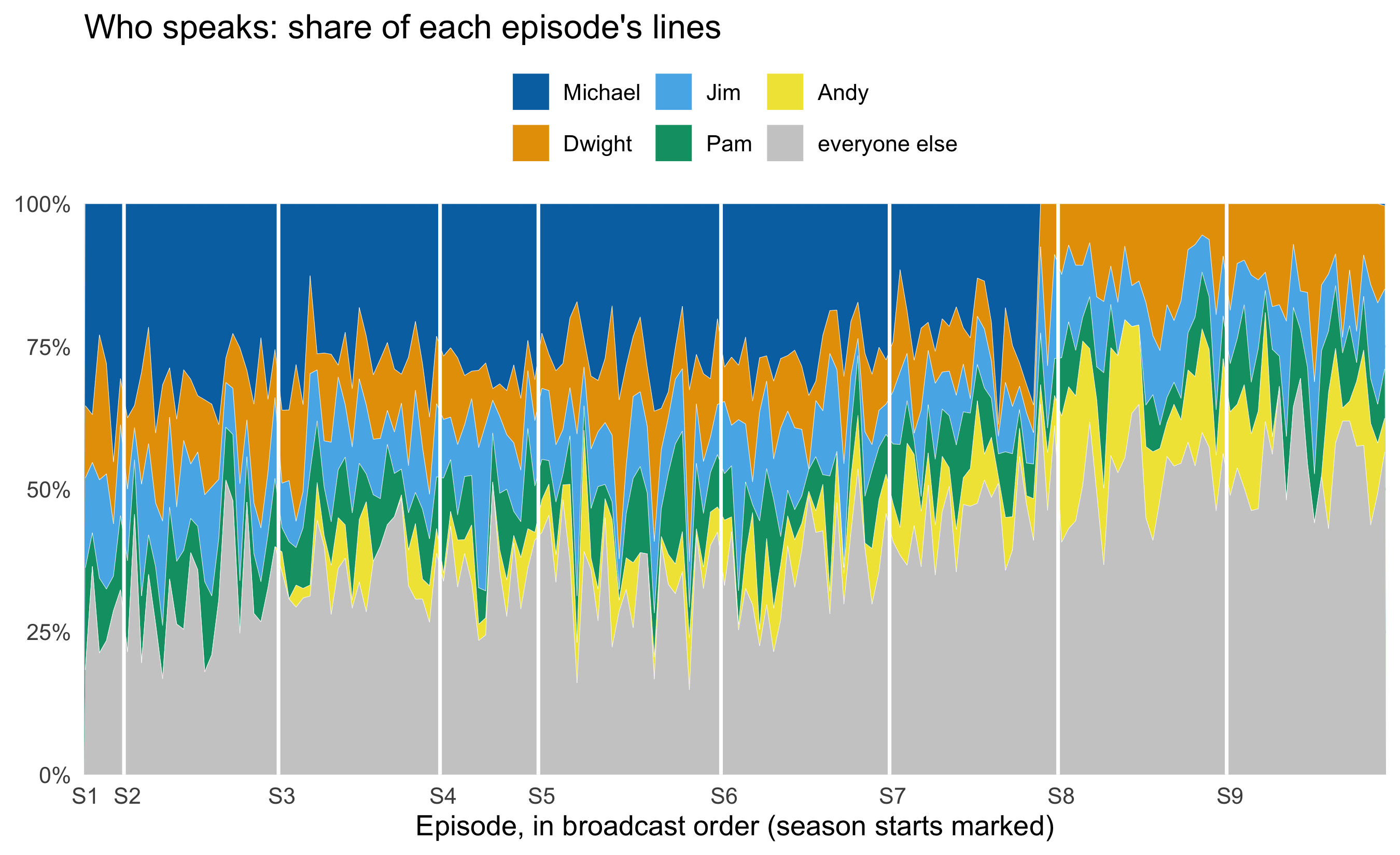
**The question the agent chose.** *The Office* started as a show about one man and became an ensemble. Can the transcripts measure that shift? And does a broader ensemble go with better or worse ratings?
In season 1, Michael speaks `r scales::percent(michael_by_season$share[1], 1)` of all lines in an average episode. By season 7, his last as a regular, that has fallen to `r scales::percent(michael_by_season$share[7], 1)`. The *effective number of speakers* is the number of equally talkative characters that would give an episode's spread of lines. It rises from `r sprintf("%.1f", eff_by_season$eff[1])` in season 1 to `r sprintf("%.1f", eff_by_season$eff[9])` in season 9.
```{r fig-ensemble-shares}
#| fig-alt: "Stacked area chart of each episode's share of spoken lines for Michael, Dwight, Jim, Pam, Andy and everyone else, across all episodes in order, with season boundaries marked."
#| fig-height: 5.5
ggplot(lead_shares, aes(x = ep_seq, y = share, fill = who)) +
  geom_area(colour = "white", linewidth = 0.1) +
  geom_vline(data = season_starts[-1, ], aes(xintercept = start - 0.5),
             colour = "white", linewidth = 0.8) +
  scale_fill_manual(values = c(unname(palette.colors(6, palette = "Okabe-Ito"))[c(6, 2, 3, 4, 5)], "grey80")) +
  scale_x_continuous(breaks = season_starts$start, labels = paste0("S", season_starts$season),
                     expand = c(0, 0)) +
  scale_y_continuous(labels = scales::percent, expand = c(0, 0)) +
  labs(title = "Who speaks: share of each episode's lines",
       x = "Episode, in broadcast order (season starts marked)", y = NULL, fill = NULL) +
  theme_minimal(base_size = 13) +
  theme(panel.grid.minor = element_blank(), legend.position = "top")
```
**Design choices (the agent's).**
- It used a stacked area of *shares*, not counts, because episodes differ in length and the question is about balance.
- The five leads are named and everyone else is pooled in grey. The transcripts have hundreds of character labels, and colour can't carry them.
- Okabe-Ito hues keep the leads distinguishable for colour-blind readers.
- White rules mark the season boundaries, and the x-axis labels sit at season starts instead of at arbitrary episode numbers.
```{r fig-ensemble-ratings}
#| fig-alt: "Scatter of IMDb rating against effective number of speakers per episode, coloured by season, with a dashed pooled regression line sloping down and flat solid lines within each season."
ggplot(breadth, aes(x = eff_speakers, y = imdb_rating)) +
  geom_point(aes(colour = factor(season)), alpha = 0.8) +
  geom_smooth(aes(colour = factor(season)), method = "lm", se = FALSE, linewidth = 0.7) +
  geom_smooth(method = "lm", se = FALSE, colour = "grey20", linetype = "dashed", linewidth = 1) +
  labs(title = "Broader ensembles, lower ratings? Only between seasons",
       x = "Effective number of speakers in the episode", y = "IMDb rating",
       colour = "Season", caption = "Dashed: one line through all episodes. Solid: one line per season.") +
  theme_minimal(base_size = 13)
```
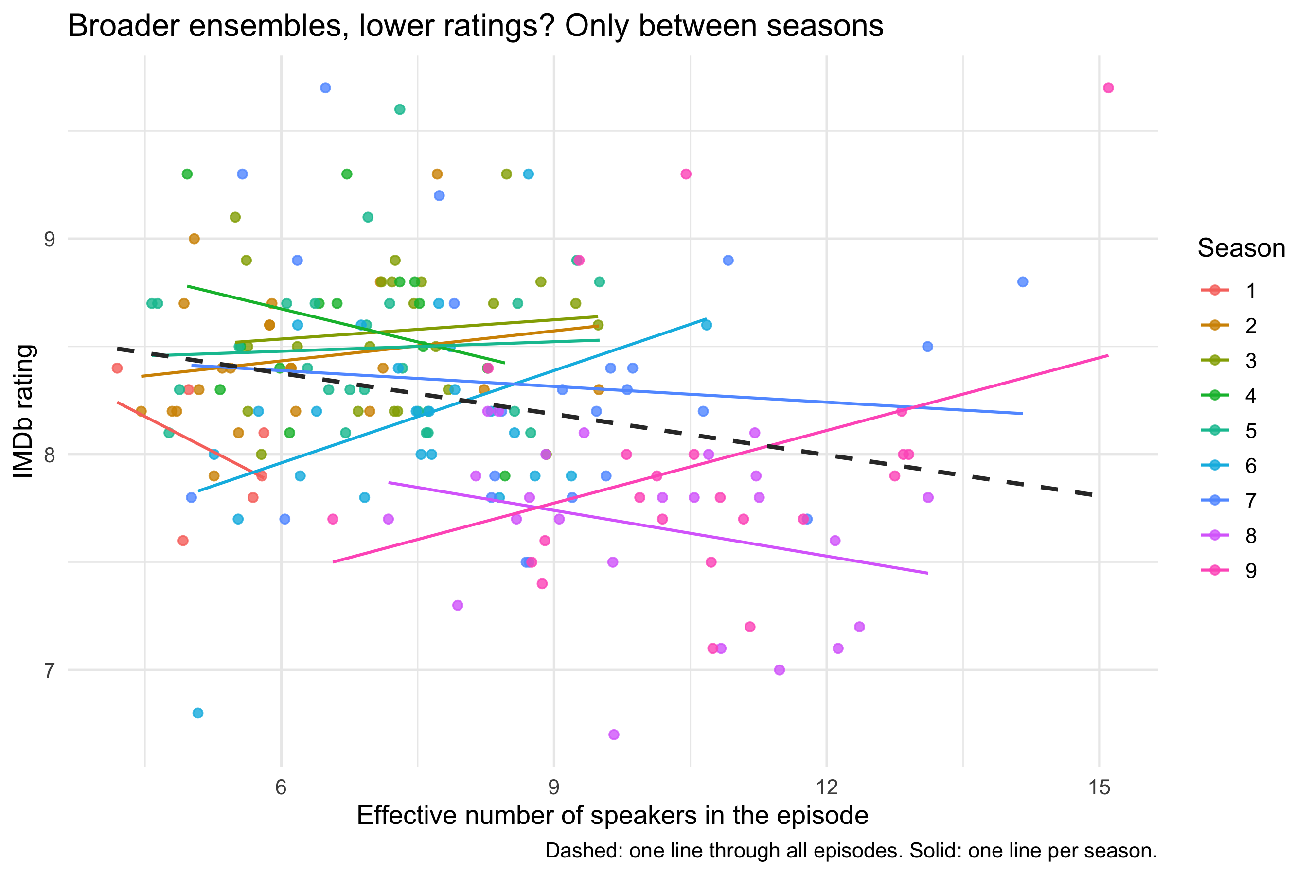
Pooled across the whole run, the effective number of speakers and the rating are negatively correlated (r = `r sprintf("%.2f", pooled_r)`). Each extra effective speaker goes with a rating `r sprintf("%.2f", abs(coef(pooled)[2]))` points lower. Give each season its own level, with `lm(imdb_rating ~ eff_speakers + factor(season))`, and the common within-season slope is `r sprintf("%+.2f", coef(within)[2])` per extra speaker (p = `r sprintf("%.2f", summary(within)$coefficients[2, 4])`), which is indistinguishable from zero. The nine season lines in the figure scatter both ways around it, with no consistent direction.
The pooled slope comes from *between*-season differences. The later seasons both spread their lines more widely and are rated lower. Nothing in the data shows that one causes the other. Michael's departure after season 7, cast and writing-staff changes, and the age of the show all shift ratings and ensemble breadth together.
**The grammar point.** The same move as spec 04 against spec 05 changes the answer: one smoother, or one per group, chosen by where a single mapping sits. With group-level confounding, the choice of layer decides whether the figure supports the claim.
## Where this fits
The workshop's central argument is that agents collapse the *implementation* part of analysis, which leaves the analyst more time for the design decisions. Knowledge Tree and Butterfly, the facilitator's company, is building this into its offering [**Science Supercharged**](https://ktandb.co.uk/ways-to-work#science-supercharged). It brings the habits software teams use to keep their work alive to research analysis: version control, specification before analysis, and checks before publication. The spec-first loop in these sessions is a small, visual instance of that. The decisions go into a file that can be reviewed, an agent does the typing, and the record of what was decided survives the session.
[*The knowledge tree*](https://ktandb.co.uk/knowledge-tree) explains the wider idea: keep alive the structure that produces an analysis, not just the outputs. The 75-second film [*A Hand of Tasks*](https://ktandb.co.uk/hand-of-tasks) frames the shift in four task types: specify, implement, review and feedback. Sessions like this one practise moving time out of *implement* and into the other three.
**How much time is at stake? Illustrative orders of magnitude, not measurements.** These estimates are deliberately low.
| Piece of work | By hand, experienced R user | Agent-assisted (human time) |
|---|---|---|
| One spec revision to a polished, labelled figure | 10–30 minutes | about 1 minute |
| This page's figures, including the 3D model view and its linked table | 1–2 days | 1–2 hours |
| Rebuilding a published paper's analysis on new data (Science Supercharged case study) | weeks | 2–3 days |
The saving is roughly an order of magnitude on implementation. Specifying, reviewing and deciding take as long as before, which is the point.
## What the data can't say
IMDb ratings come from self-selected raters voting years after broadcast, so they measure how the show is remembered by people who chose to rate it. They don't measure how it was received at the time.
The episode counts differ between tables (`r nrow(ratings)` rated episodes against `r n_ep_lines` in the transcripts). The sources likely split two-part episodes differently. Check any join for dropped rows.
The transcripts are fan-made, so character labels are inconsistent. The effective-speaker measure counts lines, not words or screen time, so a character with many one-word lines counts as much as one with a few speeches.
The 3D planes assume season acts as a number, which the group rejected for the 2D figures. They are shown to make that assumption, and its cost, visible.